Page 466 - Fiber Optic Communications Fund

Nonlinear Effects in Fibers 447

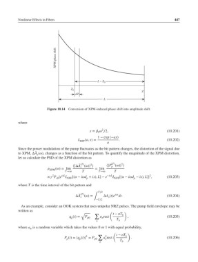
XPM phase shift

L − Z 0

Z 0
Z
dZ
L

Figure 10.14 Conversion of XPM-induced phase shift into amplitude shift.

where

2
x = ∕2, (10.201)
2
1 − exp (−ax)
L EFF (a, x)= . (10.202)
a
Since the power modulation of the pump fluctuates as the bit pattern changes, the distortion of the signal due
̃
to XPM, ΔA (), changes as a function of the bit pattern. To quantify the magnitude of the XPM distortion,
s
let us calculate the PSD of the XPM distortion as
̃ (T) 2 (T) 2
p
s
⟨|ΔA ()| ⟩ ⟨|P ()| ⟩
() = lim = lim
XPM
T→∞ T T→∞ T
2 ixL −ixL 2
× P |e L [( − id + ix), L]− e L [( − id − ix), L]| , (10.203)
s0 EFF p EFF p
where T is the time interval of the bit pattern and
T∕2
(T)
̃
it
ΔA ()= ∫ ΔA (t)e dt. (10.204)
s
s
−T∕2
As an example, consider an OOK system that uses unipolar NRZ pulses. The pump field envelope may be
written as
( )
√
∑ t − nT b
q (t)= P a rect , (10.205)
p p0 n T
n b
where a is a random variable which takes the values 0 or 1 with equal probability,
n
( )
∑ 2 t − nT b
2
P (t)= |q (t)| = P a rect . (10.206)
p p p0 n T
n b