Page 470 - Fiber Optic Communications Fund

Nonlinear Effects in Fibers 451

1

0.8

FWM efficiency 0.6

0.4

0.2

0
–2 –1 0 1 2
Dispersion (ps.ps/km)

Figure 10.16 FWM efficiency vs. for j = 1, k = 2, and l = 3. Channel spacing, Δf = 100 GHz, Ω = 2Δf, Ω =
2 1 2
4Δf, L = 80 km, loss = 0.2 dB/km, and Ω = 6Δf.
3
1

0.8
β 2 = 0.5 ps.ps/km
FWM efficiency 0.6 β = 1 ps.ps/km

0.4
2

0.2

0
0 100 200 300 400
Channel spacing (GHz)

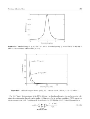
Figure 10.17 FWM efficiency vs. channel spacing, Δf. L = 80 km, loss = 0.2 dB/km, j = 1, k = 2, and l = 3.

Fig. 10.17 shows the dependence of the FWM efficiency on the channel spacing. As can be seen, the effi-
ciency decreases as the channel spacing and/or | | increases. So far we have considered FWM generation
2
due to a single triple {jkl}. Considering all the triplets in Eq. (10.208), Eq. (10.221) should be modified as
[ − jkln L ]
1 − e
∑ ∑ ∑
(L)= K jkl (10.232)
n
j k L jkln
j+k−l=n
No SPM, no XPM