Page 478 - Fiber Optic Communications Fund

Nonlinear Effects in Fibers 459

Tx. Amp Amp Amp Rx.

(a)

Power

Distance, z
(b)

α(z)

Distance, z

(c)

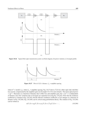
Figure 10.26 Typical fiber-optic transmission system: (a) block diagram, (b) power variation, (c) loss/gain profile.

a 2 (z)

Distance, z
L a
2
Figure 10.27 Plot of a (Z) v distance. L = amplifier spacing.
a

′
2
where Z = mod(Z, L ), where L = amplifier spacing. Fig. 10.27 shows a (Z) for a fiber-optic link with fiber
a a
loss exactly compensated by the amplifier gain (see Example 10.12 for more details). The mean optical power
2
2
< |q| > fluctuates as a function of distance due to fiber loss and amplifier gain, but < |u| > is independent
of distance since the variations due to loss/gain are separated out using Eq. (10.243). Note that the nonlinear
2
coefficient is constant in Eq. (10.242), but the effective nonlinear coefficient a (Z) changes as a function of
distance in Eq. (10.246). Eq. (10.246) can be solved using perturbation theory. The solution of Eq. (10.246)
can be written as
2
u(T, Z)= u (T, Z)+ u (T, Z)+ u (T, Z)+··· , (10.249)
2
1
0