Page 540 - Fiber Optic Communications Fund

Digital Signal Processing 521

l
(t, 0) q (t, ∆z / 2) q (t, ∆z)
q b b b
exp(D ∆z / 2) exp(∫ ∆z N (t, z)dz) exp(D ∆z / 2)
b
b
0 b
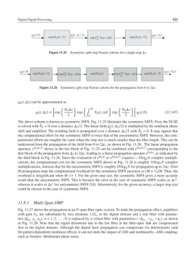
Figure 11.25 Symmetric split-step Fourier scheme for a single-step Δz.

q (t, 0) q b (t, 2∆z)
b
2∆z
N (t, z)dz)
N (t, z)dz)
b
exp(D b ∆z / 2) exp(∫ ∆z b exp(D ∆z) exp(∫ ∆z b exp(D ∆z / 2)
b
0
Figure 11.26 Symmetric split-step Fourier scheme for the propagation from 0 to 2Δz.
q (t, Δz) can be approximated as
b
[ { } { Δz } { }]
D Δz D Δz
b
b
q (t, Δz)= exp exp N (t, z)dz exp q (t, 0). (11.147)
b
b
b
2 ∫ 0 2
The above scheme is known as symmetric SSFS. Fig. 11.25 illustrates the symmetric SSFS. First, the NLSE
l
̂
is solved with N = 0 over a distance Δz∕2. The linear field q (t, Δz∕2) is multiplied by the nonlinear phase
b b
̂
shift and amplified. The resulting field is propagated over a distance Δz∕2 with N = 0. It may appear that
b
the computational effort for the symmetric SSFS is twice that of the unsymmetric SSFS. However, the com-
putational efforts are roughly the same when the step size is much smaller than the fiber length. This can be
understood from the propagation of the field from 0 to 2Δz, as shown in Fig. 11.26 . The linear propagation
operator, e b Δz∕2 shown in the last block of Fig. 11.25 can be combined with e b Δz∕2 corresponding to the
D
D
D
first block of the propagation from Δz to 2Δz, leading to a linear propagation operator e b Δz , as indicated by
D
D
the third block in Fig. 11.26. Since the evaluation of e b Δz or e b Δz∕2 requires ∼ Nlog N complex multipli-
2
cations, the computational cost for the symmetric SSFS shown in Fig. 11.26 is roughly 3Nlog N complex
2
multiplications, whereas that for the unsymmetric SSFS is roughly 2Nlog N for propagation up to 2Δz.Over
2
M propagation steps the computational overhead for the symmetric SSFS increases as (M + 1)∕M. Thus, the
overhead is insignificant when M >> 1. For the given step size, the symmetric SSFS gives a more accurate
3
result than the unsymmetric SSFS. This is because the error in the case of symmetric SSFS scales as Δz ,
2
whereas it scales as Δz for unsymmetric SSFS [24]. Alternatively, for the given accuracy, a larger step size
could be chosen in the case of symmetric SSFS.
11.8.1 Multi-Span DBP
Fig. 11.27 shows the propagation in an N-span fiber-optic system. To undo the propagation effect, amplifiers
with gain G are substituted by loss elements 1∕G in the digital domain and a real fiber with parame-
n n
ters ( , , ), n = 1, 2, … , N is replaced by a virtual fiber with parameters (− , − , − ), as shown
2n n n 2n n n
in Fig. 11.28. Note that the signal distortions due to the last fiber in the fiber-optic link are compensated
first in the digital domain. Although the digital back propagation can compensate for deterministic (and
bit-pattern-dependent) nonlinear effects, it can not undo the impact of ASE and nonlinearity–ASE coupling,
such as Gordon–Mollenauer phase noise.