Page 541 - Fiber Optic Communications Fund

522 Fiber Optic Communications

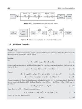
Fiber 1 Amp. 1 Fiber 2 Amp. 2 Fiber N Amp. N
q(t,0)
Tx. G 1 G 2 G N Rx. DSP
, – , – , – , – , – , – front end
2,1 1 1 2,2 2 2 2,N N N

Figure 11.27 Propagation in an N-span fiber-optic system.

DSP
virtual virtual virtual
fiber N fiber N – 1 fiber 1
IF and
Rx. Loss Loss Loss Decision
front end phase noise 1/G N – 2,N , – , – 1/G N – 1 – , – , 1/G 1 – , – , – circuit
removal N N 2,N – 1 N – 1 2,1 1 1
–
N – 1
Figure 11.28 Digital back propagation for a N-span fiber-optic system.

11.9 Additional Examples

Example 11.2

The noise n is a zero-mean complex random variable with Gaussian distribution. Show that the mean of the
l
′
effective noise n given by Eq. (11.33) is zero.
l
Solution:
Let
n = A exp (i )= A cos ( )+ iA sin ( ). (11.148)
l
l
l
l
l
l
l
Since n is a Gaussian random variable, it follows that is a random variable with uniform distribution in the
l
l
interval [0, 2]:
< n >=< A >< cos ( ) > +i < A >< sin ( ) >= 0. (11.149)
l
l
l
l
l
Consider
k
k
k
k
n = A exp (ik )= A cos (k )+ iA sin (k ), k = 1, 2, … , M (11.150)
l l l l l l l
k
k
k
< n >=< A >< cos (k ) > +i < A >< sin (k ) >= 0. (11.151)
l l l l l
Since is a uniformly distributed random variable in the interval [0, 2], k is also a uniformly distributed
l
l
random variable in the interval [0, 2k] and therefore < cos (k ) >=< sin (k ) >= 0. Eq. (11.33) may be
l
l
rewritten as
′
M
2
n = K n + K n +···+ K n , (11.152)
l 1 l 2 l M l
where K , m = 1, 2, 3, … M, are complex constants:
m
′
M
2
< n >= K < n > +K < n > +· · · + K < n >. (11.153)
l 1 l 2 l M l
k
Since < n > is zero, it follows that
l ′
< n >= 0. (11.154)
l