Page 99 - Fiber Optic Communications Fund

80 Fiber Optic Communications

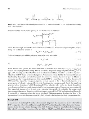
Figure 2.37 Fiber-optic system consisting of TF and DCF. TF = transmission fiber, DCF = dispersion-compensating
fiber, TX = transmitter.

transmission fiber and DCF after ignoring and fiber loss can be written as
1
[ 2 TF TF ]
i(2f) L
2
H (f)= exp ,
TF
2
[ 2 DCF DCF ]
i(2f) 2 L
H DCF (f)= exp , (2.231)
2
where the superscripts TF and DCF stand for transmission fiber and dispersion-compensating fiber, respec-
tively. The total transfer function is
H (f)= H (f)H (f). (2.232)
tot TF DCF
To keep the output pulse width equal to the input pulse width, we require

H (f)= 1, (2.233)
tot
or
TF TF
L =− DCF DCF . (2.234)
L
2 2
L
When the loss is not ignored, the output of the DCF is attenuated by a factor exp [− L − DCF DCF ]
TF TF
TF TF
without affecting the pulse broadening. When is included, the pulse is simply delayed by a factor L +
1
1
L
DCF DCF . Typically, SSMFs or NZDSFs are used as transmission fibers, which have anomalous dispersion.
1
Therefore, the DCF should have normal dispersion. As mentioned before, the fiber dispersion coefficient can
be altered by changing the amount of waveguide dispersion. The material dispersion of glass at 1550 nm is
anomalous and the waveguide dispersion of the standard SMF is a small fraction of the total dispersion (at
1550 nm). If the sign of the waveguide dispersion is made opposite to that of the material dispersion by a
proper choice of refractive index profile, the total fiber dispersion becomes normal. This is the underlying
principle behind the design of a DCF. To design a DCF, the refractive index profile of a fiber is divided into
several segments. Each segment is characterized by two or more parameters. For example, a segment could
have a parabolic index profile or it could have a triangular index profile. By optimizing the parameters of
these segments, the desired dispersion coefficient can be obtained. For WDM applications (see Chapter 9),
2
it is desirable to compensate dispersion over a wide band. With proper design, the dispersion slope of the
transmission fiber can also be compensated [41]. Such a fiber is called a dispersion-slope compensating fiber.
Example 2.11
2
A transmission fiber of length 80 km has a dispersion of −21 ps /km. The transmission fiber is followed by a
2
DCF of dispersion 130 ps /km. (a) Find the length of the DCF such that the pulse width at the input of the trans-
mission fiber is the same as that at the output of the DCF. (b) Suppose the power launched into the transmission
fiber is 2 mW, losses of the transmission fiber and DCF are 0.2 dB/km and 0.5 dB/km, respectively. Calculate