Page 66 - Instrumentation and Measurement

Answer:

a. Using the equation:

controller output = Kp (error + (1/Ti) x integral of error + Td x rate of change of error)

we have for time t = 0 an error of 0, a rate of change of error with time of 1 s-1, and an area between
this value of t and t = 0 of 0. Thus

b. When t = 2 s, the error has become 1%, the rate of change of the error with time is 1%/s and the
area under between t = 2 and t = 0 is 1%/s. Thus

controller output = 4 (1 + (1/0.2) x 1 + 0.5 x 1) = 26%

4.8 Tuning

The design of a controller for a particular situation involves selecting the control modes to be used
and the control mode settings. This means determining whether proportional control, proportional
plus derivative, proportional plus integral or proportional plus integral plus derivative is to be used
and selecting the values of KP, Ki and Kd. These determine how the system reacts to a disturbance or
a change in the set value, how fast it will respond to changes, how long it will take to settle down
after a disturbance or change to the set value, and whether there will be a steady state error.

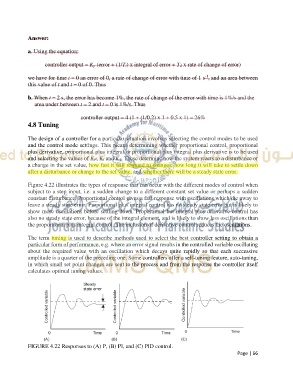
Figure 4.22 illustrates the types of response that can occur with the different modes of control when
subject to a step input, i.e. a sudden change to a different constant set value or perhaps a sudden
constant disturbance. Proportional control gives a fast response with oscillations which die away to
leave a steady state error. Proportional plus integral control has no steady state error but is likely to
show more oscillations before settling down. Proportional but integral plus derivative control has
also no steady state error, because of the integral element, and is likely to show less oscillations than
the proportional plus integral control. The inclusion of derivative control reduces the oscillations.

The term tuning is used to describe methods used to select the best controller setting to obtain a
particular form of performance, e.g. where an error signal results in the controlled variable oscillating
about the required value with an oscillation which decays quite rapidly so that each successive
amplitude is a quarter of the preceding one. Some controllers offer a self-tuning feature, auto-tuning,
in which small set point changes are sent to the process and from the response the controller itself
calculates optimal tuning values.

FIGURE 4.22 Responses to (A) P, (B) PI, and (C) PID control.

Page | 66