Page 22 - tmp_Neat

involving heavy vehicles. Milton et al. (2008) developed a mixed logit model with severity

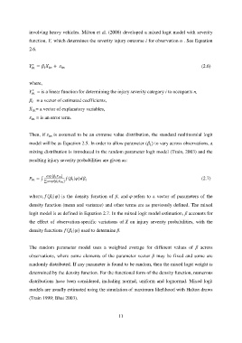
function, Y, which determines the severity injury outcome i for observation n . See Equation
2.6.

(2.6)

where,

= is a linear function for determining the injury severity category i to occupants n,

= a vector of estimated coefficients,

= a vector of explanatory variables,

= is an error term.

Then, if is assumed to be an extreme value distribution, the standard multinomial logit

model will be as Equation 2.5. In order to allow parameter ( ) to vary across observations, a

mixing distribution is introduced in the random parameter logit model (Train, 2003) and the
resulting injury severity probabilities are given as:

∫ [ ] ( | ) (2.7)

∑ [ ]

( | ) is the density function of β, and refers to a vector of parameters of the

density function (mean and variance) and other terms are as previously defined. The mixed

logit model is as defined in Equation 2.7. In the mixed logit model estimation, β accounts for
the effect of observation-specific variations of on injury severity probabilities, with the

density functions ( | ) used to determine β.

The random parameter model uses a weighted average for different values of β across

observations, where some elements of the parameter vector β may be fixed and some are
randomly distributed. If any parameter is found to be random, then the mixed logit weight is

determined by the density function. For the functional form of the density function, numerous
distributions have been considered, including normal, uniform and lognormal. Mixed logit

models are usually estimated using the simulation of maximum likelihood with Halton draws
(Train 1999; Bhat 2003).

11