Page 2 - artt

Advances in Social Science, Education and Humanities Research, volume 176

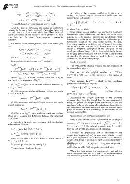
(0) (1) (0) (2) (0) () According to the relational coefficient G () between
0
(1) () = ( , , . . . . . . , ) factors, the relevant degree between each child factor and
(0) (1) (0) (1) (0) (1)
mother factor is obtained:
= ( (1) (1) , (1) (2), . . . . . . , (1) () ) 1
= ∑ G () (i = 1 , 2 , 3 , . . . . . . , n ; k = 1 ,
0
0
The establishment of relevant degree analysis model =1
2 , 3 , . . . . . . ,n)
After the data is initialized, the degree of correlation
between the factors is further analyzed. The mother factor and B. Gray Forecast Model
the child factor need to be determined here. Then the trend Gray relevant degree analysis can analyze the correlation
curve consistency of the sequence curve geometry of each between the known child factors and the mother factor in the
child factor and the mother factor sequence geometry is system, so as to roughly simulate the development trend
compared. between the child factor and the mother factor. There is a grey
forecasting model in the gray model system. The grey
Let mother factor series ()and child factor series () forecasting model is to establish a grey differential forecasting

0
be: model with a small amount of incomplete information, and
() = ( (1), (2), . . . . . . , ()) makes a long-term description of the ambiguity of the
0
0
0
0
development law of things [10]. Its characteristic is that the use
() = ( (1), (2), . . . . . . , ()) of the gray prediction model does not require a large number

of samples, the sample does not need to have a regular
(i = 1, 2, . . . . . . , n; j = 1,2, . . . . . . , m); distribution, and the accuracy is high.
Relational coefficient between () and (): Model processing:

0
G () The setting of the original sequence and the generation of
0

the accumulated sequence
0

0

| () − ()| + p | () − ()|
= First we set the original number to (0) () =
| () − ()| + p | () − ()| ( (0) (1), (0) (2), . . . . . . , (0) () )(where n is the number of
0

0
Where G () is called the relational coefficient of to data)
0
0
at time i, in the expression ofG (): Then initialize the (0) () , which is the cumulative

0
generation of the original sequence:
(2.1)| () − ()| is the absolute difference between
0
0

and at time i (1) () = ∑ =1 (0) () (t=1, 2, 3,……, n)

(2.2)The minimum absolute difference between two levels Then get (1) (), (1) () =
at each moment is: ( (1) (1), (1) (2), … . . . (1) ());
Accumulate the weight coefficient of the generated
∆ = | () − ()| sequence obeys Yang Hui triangle law, the more accumulated
0

(2.3)The maximum absolute difference between two levels times, the greater the weight of old settlements, so that the
at each moment is: number of columns after accumulation is changed according to
the monotonous ascending rule of the Yanghui triangle, which

∆ = | () − ()| plays an essential role in weakening the randomness of the

0
original sequence[12].
(2.4)The p in G () is the resolution coefficient, and the
0
effect is to increase the difference between the relational Quasi-smooth test and Quasi-exponential test
coefficients.
First, a quasi-smooth check is performed on the original
pvalue rule is: Note that ∆ is the mean of all the absolute sequence (0) () , constructing p(t) = (0) () ,(k = 2 ,

values of the difference: (1) (−1)
3 , ……, n), p(t) ∈ [0 ],when k is greater than 3, if <0.5,
1
∆ = ∑ ∑ | () − ()|, then we call (0) () as a quasi-smooth sequence.
0

∗ =1 =1
Secondly, the exponential test is performed on the
= ∆ , then the value of p is: (1) (1)
∆
∆ accumulated sequence (). In order to test whether ()
when ∆ > 3∆ , ≤ p ≤ 1.5 ∆ ; when ∆ ≤ has a quasi-exponential law, a formula that can quantitatively
∆
3∆ , 1.5 ≤ p ≤ 2 , describe the degree of coincidence has been introduced:σ(t) =
∆

∆
(1) ()
In general, p takes (0.1, 1), usually 0.5. (1) (−1) ,(k= 2 , 3 ,……,n),σ(t) ∈ [1 1 + ],when kis greater 3,
The calculation of relevant degree <0.5, then we call (0) () as quasi-exponential law。
When the data passes the quasi-smooth test and the
quasi-exponential test, the grey GM (1, 1) prediction model
can be used for quantitative prediction and calculation.
436