Page 5 - artt

Advances in Social Science, Education and Humanities Research, volume 176

A quasi-smoothing test is performed on the original (1) ( + 1) = [ (0) (1) − ] − +
series (0) , and the original series can satisfy the quasi-smooth
sequence when t=4. As shown in Table 5: (1) 0.1063
( + 1) = 2141.07 − 1972.92 (t= 0, 1,
2,……,)
TABLE V QUASI-SMOOTHNESS TEST
According to the time-response formula, the corresponding
t 4 5 6 7 8
cumulative forecast of tourism comprehensive income for
P(t) 0.48772 0.34027 0.28609 0.25151 0.22574 Huangshan City from 2009 to 2016 can be calculated
separately.
A quasi-exponential test is performed on the accumulated
(1)
series (1) , and the accumulated series can be obtained as t=4 ̂ ()
to satisfy the quasi-smooth sequence. As shown in Table 6: = (168.15, 408.28, 675.35, 972.37, 1302.70, 1670.07,
2078.66, 2533.06)
TABLE VI QUASI-EXPONENTIAL TEST
(0)
(1)
(1)
t 4 5 6 7 8 From ̂ () = ̂ ( + 1) − ̂ () , the predicted
values for each year can be calculated separately, as shown in
() 1.48773 1.34028 1.2861 1.25151 1.22574 Table 7:
Do the adjacent data column processing for (1) ():
TABLE VII PREDICTED RESULTS
(1) () = (772.75; 1081.5; 1415.95; 1793.5; 2218.9) t 1 2 3 4 5 6 7 8
Least squares estimation of parameter ̂ = [, ] and 168 240 267 297 330 367 408 454

()
calculate: ̂ ()) .15 .13 .06 .02 .33 .38 .58 .41

̂ = [, ] = (−0.1063,209.7215) Using MATLAB, the results of the operation (predicted

Bring in coefficients to determine differential equations values) are compared and analyzed with the results (actual
values) of the present values. The predicted and actual curves
(1) are shown. As shown in Figure 1 below:
− 0.1063 (1) = 209.7215

Find the solution of the differential equation and get the
time response:

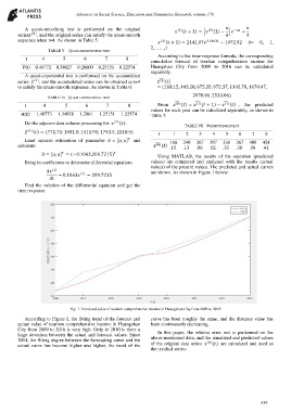
Fig. 1 Trend and value of tourism comprehensive income of Huangshan City from 2009 to 2016

According to Figure 1, the fitting trend of the forecast and curve has been roughly the same, and the distance value has
actual value of tourism comprehensive income in Huangshan been continuously decreasing.
City from 2009 to 2016 is very high. Only in 2010 is there a
large deviation between the actual and forecast values. Since In this paper, the relative error test is performed on the
2014, the fitting degree between the forecasting curve and the above-mentioned data, and the simulated and predicted values
(0)
actual curve has become higher and higher, the trend of the of the original data series () are calculated and used as
the residual series:

439