Page 214 - Six Sigma Advanced Tools for Black Belts and Master Black Belts

Char Count= 0
2:58
August 31, 2006
JWBK119-13
Confidence Limits for k 199
10 −1 0.75
0.7
−2
10
0.6
10 −3 0.5
10 −4
0.4
10 −5
P 0.3
10 −6
10 −7 0.2
10 −8
10 −9 0.1
10 −10
k = 0
0.7 0.8 0.9 1.0 1.1 1.2 1.3 1.4 1.5 1.6 1.7 1.8 1.9 2.0 2.1 2.2
C p

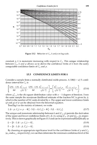
Figure 13.2 Behavior of C p , k and p on log scale.

constant p, k is monotonic increasing with respect to C p . This unique relationship
between C p , k and p allows us to derive the confidence limits of k from the easily
computable confidence limits of C p and p.

13.3 CONFIDENCE LIMITS FOR k

Consider a sample from a normally distributed stable process. A 100(1 − α) % confi-
dence interval for C p is
2 2 2 2
USL−LSL χ n−1,α/2 USL−LSL χ n−1,1−α/2 χ n−1,α/2 χ n−1,1−α/2
ˆ
ˆ
√ , √ ≡ √ C p , √ C p , (13.6)
6ˆσ n−1 6ˆσ n−1 n−1 n−1
where χ 2 is the chi-square distribution value with n − 1 degrees of freedom. From
n−1
the same sample the maximum likelihood estimate of the fraction NC is given by ˆp,
which is the number of NC units divided by n. The upper and lower confidence limits
(¯p and p)of ˆp can be obtained from the binomial equation.
Treating k as the statistic of interest, we write

L (k : p, C p ) = p − −3 (1 + k) C p + −3 (1 − k) C p . (13.7)
The unique and monotonic relationship between k and (C p , p) permits the derivation
¯
¯
of the upper and lower confidence limits of k,(k, k), using (C p , ¯p) and (C , p), respec-
p
tively. This is shown graphically in Figure 13.3 and can be expressed mathematically as

k = k : L (k : p, C p ) = 0 , (13.8)
¯ k = k : L (k :¯p, C p ) = 0 . (13.9)
¯

By choosing an appropriate significance level for the confidence limits of p and C p
, respectively), we can then determine the minimum confidence level of the
(α p and α C p