Page 215 - Six Sigma Advanced Tools for Black Belts and Master Black Belts

2:58
August 31, 2006
Char Count= 0
JWBK119-13
200 A Graphical Approach to Obtaining Confidence Limits of C pk

p
k

p

P
k

C p C p
C p

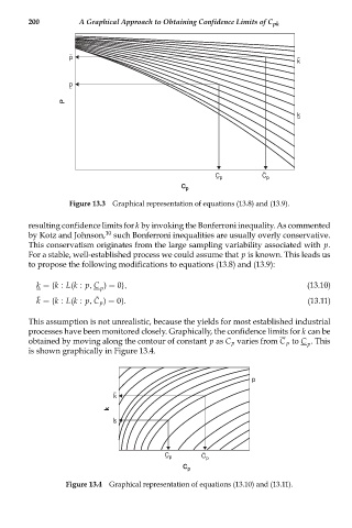
Figure 13.3 Graphical representation of equations (13.8) and (13.9).

resulting confidence limits for k by invoking the Bonferroni inequality. As commented
10
by Kotz and Johnson, such Bonferroni inequalities are usually overly conservative.
This conservatism originates from the large sampling variability associated with p.
For a stable, well-established process we could assume that p is known. This leads us
to propose the following modifications to equations (13.8) and (13.9):

k ={k : L(k : p, C ) = 0}, (13.10)
p
¯
¯
k ={k : L(k : p, C p ) = 0}. (13.11)
This assumption is not unrealistic, because the yields for most established industrial
processes have been monitored closely. Graphically, the confidence limits for k can be
obtained by moving along the contour of constant p as C p varies from C p to C . This
p
is shown graphically in Figure 13.4.

p
k
k
k

C p C p
C p
Figure 13.4 Graphical representation of equations (13.10) and (13.11).