Page 285 - Six Sigma Advanced Tools for Black Belts and Master Black Belts

OTE/SPH
OTE/SPH
August 31, 2006
JWBK119-18
Taguchi Methods
270 3:6 Char Count= 0

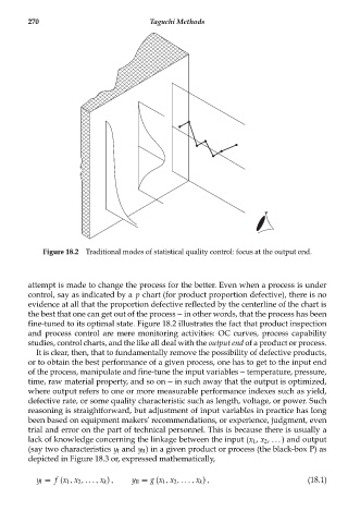
Figure 18.2 Traditional modes of statistical quality control: focus at the output end.

attempt is made to change the process for the better. Even when a process is under
control, say as indicated by a p chart (for product proportion defective), there is no
evidence at all that the proportion defective reflected by the centerline of the chart is
the best that one can get out of the process -- in other words, that the process has been
fine-tuned to its optimal state. Figure 18.2 illustrates the fact that product inspection
and process control are mere monitoring activities: OC curves, process capability
studies, control charts, and the like all deal with the output end of a product or process.
It is clear, then, that to fundamentally remove the possibility of defective products,
or to obtain the best performance of a given process, one has to get to the input end
of the process, manipulate and fine-tune the input variables -- temperature, pressure,
time, raw material property, and so on -- in such away that the output is optimized,
where output refers to one or more measurable performance indexes such as yield,
defective rate, or some quality characteristic such as length, voltage, or power. Such
reasoning is straightforward, but adjustment of input variables in practice has long
been based on equipment makers’ recommendations, or experience, judgment, even
trial and error on the part of technical personnel. This is because there is usually a
lack of knowledge concerning the linkage between the input (x 1 , x 2 , . . . ) and output
(say two characteristics y I and y II ) in a given product or process (the black-box P) as
depicted in Figure 18.3 or, expressed mathematically,

y I = f (x 1 , x 2 ,..., x k ) , y II = g (x 1 , x 2 ,..., x k ) , (18.1)