Page 294 - Six Sigma Advanced Tools for Black Belts and Master Black Belts

OTE/SPH
OTE/SPH
Char Count= 0
August 31, 2006
JWBK119-18
3:6
Taguchi’s ‘Statistical Engineering’ 279
y

Δy ′=Δy 1 Δy 2 y 2
2

Δy ′=Δy 1 y 1
2

x
x 1 x 2
Δx Δx
Δx′
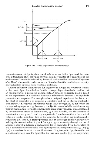
Figure 18.8 Effect of parameter x on response y.

parameter--noise relationship is revealed to be as shown in this figure and the value
*
of x d is then fixed at x , the value of y will from now on stay at y * regardless of the
d
environmental condition reflected by the actual (and in real life uncontrollable) value
of x e . Thus ‘robustness’in performance is achieved without the need to invest in costly
new technology or better noise-resistance materials.
Another important consideration for engineers in design and operation studies
is direct cost. Apart from the loss function concept, Taguchi methods consider cost
an integral part of a parameter design study. A strategy frequently cited is based
on the exploitation of a nonlinear functional relationship between a manipulable
parameter and response. For example, after a designed experiment has been run,
the effect of parameter x on response y is isolated and can be shown graphically
as in Figure 18.8. Suppose the nominal design value is originally x 1 , for which the
corresponding response is y 1 . Because x 1 is subject to uncontrollable variation during
product manufacture (owing to component-to-component variation) or usage (caused
by environmental stress or deterioration), y 1 is also variable, and the amounts of
variation for x and y are x and y, respectively. It can be seen that if the nominal
value of x is set at x 2 instead, then for the same x, the variation in y is substantially
reduced to y 2 . Thus x 2 is greatly preferred to x 1 in the design, as it is relatively easy
to bring the nominal value of y back from y 2 to y 1 subsequently through the use of
a linear relationship between y and another design parameter. Even if a variation of

y 1 is acceptable when compared with a given performance specification y 2 ( y 2 ≤
y 1 ), x should not be set at x 1 : as an illustration, if y is equal to y 1 , then with x set

2
at x 2 , it can be seen from the figure that the hardware needed (e.g. the temperature