Page 247 - Maxwell House

Chapter 5 227

somewhat unusual units [dBW] being calculated as the arithmetic product of antenna gain in
[dBi] and transmitter power in [W]. Then the power of the wave intercepted by the receiving

antenna and delivered to the receiver input is proportional to the receiving antenna efficiency
and its effective aperture

2
2
= = = � � � � = 2 = (5.61)

2 2
4 2 4 2 4 �4 �
Here and is the effective aperture of the receiving and transmit antenna, respectively. As

expected, the intercepted power goes up very fast ~ as frequency increases while all other
2

parameters are constant. That is why high-speed wireless communication systems supporting a
5G standard are making a slow but inevitable shift to mm-wave frequency range above 24 GHz
( < 1.25 mm) to accommodate the increases in data usage. The equity (5.61) is known as the
basic Friis Transmission Formula and one of the fundamental equations of antenna theory. The
ratio expressed in dB
= 10log( ) [dB] (5.62)
⁄

describes the free-space path loss in the transmitted signal strength. Applying (5.62) to (5.61)
we obtain
= [dBi] + [dBi] − 20log() − 20log() + 147.558 [dB] (5.63)

Here in [m], f = c / in [Hz], and c = 3⋅ 10 [m/s]. Note that 147.558 = 20log10(/4).
8
In general, the receiver recognizes the transmitted signal if its power exceeds the receiver noise
threshold equal to = ∆ where is the receive noise temperature and ∆ is the

receiver bandpass. If so, some margin in signal power shall be designated for link stability as
2
2 ∆ 4
Margin = 2 − ∆ and > � � (5.64)

�4 �
It is convenient to represent the inequity in (5.64) in [dB]
[dBi] + [dBi] > 20log() + 10log( ∆) + 10log( ) − 10log( ) − 376.16 (5.65)
2

It is worthwhile to point out that the path loss estimations in (5.64) and (5.65) are quite
optimistic because they do not include such phenomena as polarization mismatch, path
obstruction by buildings and other physical objects, scattering due to woodland and
mountainous terrain, atmospheric absorption (fog, rain, hail, snow, etc.), outdoor-to-indoor loss

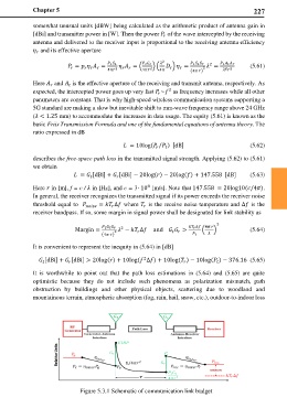
Figure 5.3.1 Schematic of communication link budget