Page 49 - Maxwell House

BASIC EQUATIONS OF MACROSCOPIC ELECTRODYNAMICS 29

the space free of field sources ( = 0). Note that (1.41) is the well-known law of

electromagnetic induction

Φ ()
ℰ() = − (1.42)

discovered by Michael Faraday in 1831. Here the ElectroMotive Force (EMF) ℰ() =
∮ ∘ in Volts or and the magnetic field flux Φ () = ∬ ∘ . The minus sign is an

indication that the electric potential in such a direction as to produce a current flux. Added to
the original flux, it would reduce the magnitude of the potential. This statement that induced
voltage acts to produce an opposing flux is known as Lenz’s law.
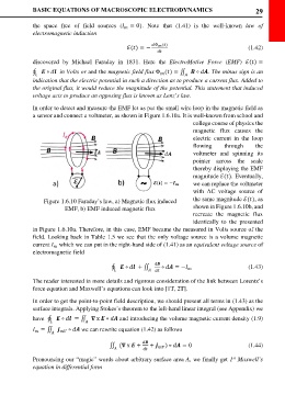
In order to detect and measure the EMF let us put the small wire loop in the magnetic field as
a sensor and connect a voltmeter, as shown in Figure 1.6.10a. It is well-known from school and
college course of physics the
magnetic flux causes the
electric current in the loop
flowing through the
voltmeter and spinning its
pointer across the scale
thereby displaying the EMF
magnitude ℰ(). Eventually,
we can replace the voltmeter
with AC voltage source of
Figure 1.6.10 Faraday’s law, a) Magnetic flux induced the same magnitude ℰ(), as
EMF, b) EMF induced magnetic flux shown in Figure 1.6.10b, and
recreate the magnetic flux
identically to the presented
in Figure 1.6.10a. Therefore, in this case, EMF became the measured in Volts source of the
field. Looking back in Table 1.5 we see that the only voltage source is a volume magnetic
current which we can put in the right-hand side of (1.41) as an equivalent voltage source of

electromagnetic field

∮ ∘ + ∬ ∘ = − (1.43)

The reader interested in more details and rigorous consideration of the link between Lorentz’s
force equation and Maxwell’s equations can look into [1T, 2T].

In order to get the point-to-point field description, we should present all terms in (1.43) as the
surface integrals. Applying Stokes’s theorem to the left-hand linear integral (see Appendix) we
have ∮ ∘ = ∬ x ∘ and introducing the volume magnetic current density (1.9)

= ∬ ∘ we can rewrite equation (1.42) as follows

) ∘ = 0 (1.44)
∬ ( x + +

Pronouncing our “magic” words about arbitrary surface area A, we finally get 1 Maxwell’s
st
equation in differential form