Page 144 - Fundamentals of Management Myths Debunked (2017)_Flat

Exhibit QM–3 Quantitative Module 143

Strong $320,000 Expected value (in 000s)
.70
.70 [320] + .30 [50] = 239
Rent
20,000 sq. ft. Weak

.30 $50,000 No expansion
1 2 Add 4,000
Strong $240,000
.70 Add 8,000
Rent
12,000 sq. ft.
Expected value (in 000s)
Weak
.30 $130,000 .70 [240] + .30 [130] = 207
= Decision point
= Outcome point

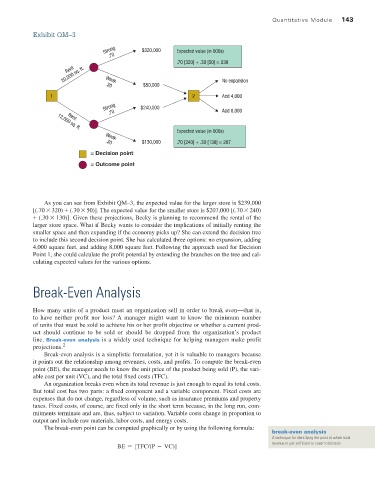
As you can see from Exhibit QM–3, the expected value for the larger store is $239,000
[(.70 * 320) + (.30 * 50)]. The expected value for the smaller store is $207,000 [(.70 * 240)
+ (.30 * 130)]. Given these projections, Becky is planning to recommend the rental of the
larger store space. What if Becky wants to consider the implications of initially renting the
smaller space and then expanding if the economy picks up? She can extend the decision tree
to include this second decision point. She has calculated three options: no expansion, adding
4,000 square feet, and adding 8,000 square feet. Following the approach used for Decision
Point 1, she could calculate the profit potential by extending the branches on the tree and cal-
culating expected values for the various options.

Break-Even Analysis

How many units of a product must an organization sell in order to break even—that is,
to have neither profit nor loss? A manager might want to know the minimum number
of units that must be sold to achieve his or her profit objective or whether a current prod-
uct should continue to be sold or should be dropped from the organization’s product
line. Break-even analysis is a widely used technique for helping managers make profit
projections. 2
Break-even analysis is a simplistic formulation, yet it is valuable to managers because
it points out the relationship among revenues, costs, and profits. To compute the break-even
point (BE), the manager needs to know the unit price of the product being sold (P), the vari-
able cost per unit (VC), and the total fixed costs (TFC).
An organization breaks even when its total revenue is just enough to equal its total costs.
But total cost has two parts: a fixed component and a variable component. Fixed costs are
expenses that do not change, regardless of volume, such as insurance premiums and property
taxes. Fixed costs, of course, are fixed only in the short term because, in the long run, com-
mitments terminate and are, thus, subject to variation. Variable costs change in proportion to
output and include raw materials, labor costs, and energy costs.
The break-even point can be computed graphically or by using the following formula:
break-even analysis
A technique for identifying the point at which total
revenue is just sufficient to cover total costs
BE = [TFC/(P - VC)]