Page 702 - Krugmans Economics for AP Text Book_Neat

enough time has elapsed for firms to enter or exit the industry. To analyze monopolis-
tic competition, we focus first on the short run and then on how an industry moves
from the short run to the long run.
Panels (a) and (b) of Figure 67.1 show two possible situations that a typical firm in a
monopolistically competitive industry might face in the short run. In each case, the
firm looks like any monopolist: it faces a downward-sloping demand curve, which im-
plies a downward-sloping marginal revenue curve.
We assume that every firm has an upward-sloping marginal cost curve but that it
also faces some fixed costs, so that its average total cost curve is U-shaped. This as-
sumption doesn’t matter in the short run; but, as we’ll see shortly, it is crucial to under-
standing the long-run equilibrium.
In each case the firm, in order to maximize profit, sets marginal revenue equal to
marginal cost. So how do these two figures differ? In panel (a) the firm is profitable; in
panel (b) it is unprofitable. (Recall that we are referring always to economic profit and
not accounting profit—that is, a profit given that all factors of production are earning
their opportunity costs.)
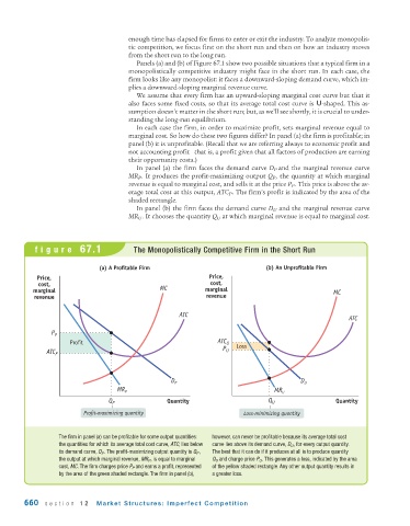
In panel (a) the firm faces the demand curve D P and the marginal revenue curve
MR P . It produces the profit-maximizing output Q P , the quantity at which marginal
revenue is equal to marginal cost, and sells it at the price P P . This price is above the av-
erage total cost at this output, ATC P . The firm’s profit is indicated by the area of the
shaded rectangle.
In panel (b) the firm faces the demand curve D U and the marginal revenue curve
MR U . It chooses the quantity Q U at which marginal revenue is equal to marginal cost.

figure 67.1 The Monopolistically Competitive Firm in the Short Run

(a) A Profitable Firm (b) An Unprofitable Firm
Price, Price,
cost, cost,
marginal MC marginal MC
revenue revenue

ATC
ATC

P P
Profit ATC U Loss
P U
ATC P

D P D U
MR P MR U
Q P Quantity Q U Quantity
Profit-maximizing quantity Loss-minimizing quantity

The firm in panel (a) can be profitable for some output quantities: however, can never be profitable because its average total cost
the quantities for which its average total cost curve, ATC, lies below curve lies above its demand curve, D U , for every output quantity.
its demand curve, D P . The profit-maximizing output quantity is Q P , The best that it can do if it produces at all is to produce quantity
the output at which marginal revenue, MR P , is equal to marginal Q U and charge price P U . This generates a loss, indicated by the area
cost, MC. The firm charges price P P and earns a profit, represented of the yellow shaded rectangle. Any other output quantity results in
by the area of the green shaded rectangle. The firm in panel (b), a greater loss.

660 section 12 Market Structures: Imperfect Competition