Page 22 - u4

QC: OSO/OVY
P2: OSO/OVY
T1: OSO
P1: OSO/OVY
July 4, 2016
GO01962-Smith-v1.cls
UAE_Math_Grade_12_Vol_1_SE_718383_ch3
13:38
Using (1.5) and (1.6), we get
f(8.02) ≈ f(8) + dy = 2 + 1 ≈ 2.0016667,
600
√
while your calculator accurately returns 3 8.02 ≈ 2.0016653. Similarly, we get
1 −2∕3
x Error f(8.07) ≈ f(8) + 8 (8.07 − 8) ≈ 2.0058333
8.02 1.4 × 10 −6 3
8.07 1.7 × 10 −5 and f(8.15) ≈ f(8) + 8 (8.15 − 8) ≈ 2.0125,
1 −2∕3
8.15 7.7 × 10 −5 3
Error in linear approximation √ √
3
3
while your calculator returns 8.07 ≈ 2.005816 and 8.15 ≈ 2.01242. In the
margin, we show a table with the error in using the linear approximation to
approximate √ x. Note how the error grows large as x gets farther from 8.
3
√
3
To approximate 25.2, observe that 8 is not the closest number to 25.2 whose
y cube root we know exactly. Since 25.2 is much closer to 27 than to 8, we write
f(25.2) = f(27) +Δy ≈ f(27) + dy = 3 + dy.
2 In this case,
( )
′
dy = f (27)Δx = 1 27 −2∕3 (25.2 − 27) = 1 1 (−1.8) =− 1
3 3 9 15
x and we have f(25.2) ≈ 3 + dy = 3 − 1 ≈ 2.9333333,
8 15
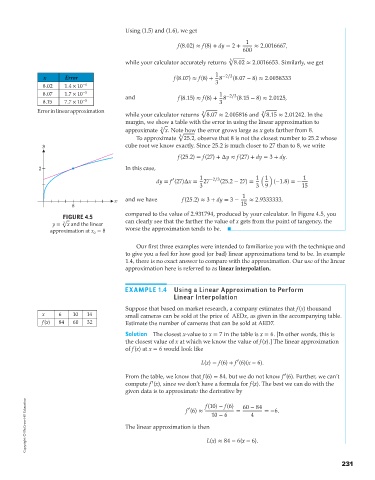
compared to the value of 2.931794, produced by your calculator. In Figure 4.5, you
FIGURE 4.5
y = √ x and the linear can clearly see that the farther the value of x gets from the point of tangency, the
3
approximation at x = 8 worse the approximation tends to be.
0
Our first three examples were intended to familiarize you with the technique and
to give you a feel for how good (or bad) linear approximations tend to be. In example
1.4, there is no exact answer to compare with the approximation. Our use of the linear
approximation here is referred to as linear interpolation.

EXAMPLE 1.4 Using a Linear Approximation to Perform
Linear Interpolation
Suppose that based on market research, a company estimates that f(x) thousand
x 6 10 14 small cameras can be sold at the price of AEDx, as given in the accompanying table.
f(x) 84 60 32 Estimate the number of cameras that can be sold at AED7.
Solution The closest x-value to x = 7 in the table is x = 6. [In other words, this is
the closest value of x at which we know the value of f(x).] The linear approximation
of f(x) at x = 6 would look like

′
L(x) = f(6) + f (6)(x − 6).
′
From the table, we know that f(6) = 84, but we do not know f (6). Further, we can’t
′
compute f (x), since we don’t have a formula for f(x). The best we can do with the
given data is to approximate the derivative by 60 − 84
Copyright © McGraw-Hill Education The linear approximation is then L(x) ≈ 84 − 6(x − 6). =−6.
f(10) − f(6)
′
f (6) ≈
=
10 − 6
4

231