Page 65 - u4

P2: OSO/OVY
P1: OSO/OVY
17:24
GO01962-Smith-v1.cls
UAE-Math-Grade-12-Vol-1-SE-718383-ch4
4-45 QC: OSO/OVY T1: OSO October 25, 2018 SECTION 4.5 • • Concavity and the Second Derivative Test 255
y y
x
-2 -1 1 2
4
-2

2
-4
x
-2 -1 1 2
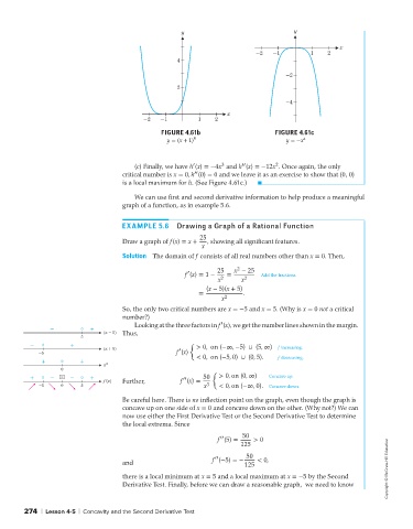
FIGURE 4.61b FIGURE 4.61c
y = (x + 1) 4 y =−x 4

′′
′
3
2
(c) Finally, we have h (x) =−4x and h (x) =−12x . Once again, the only
′′
critical number is x = 0,h (0) = 0 and we leave it as an exercise to show that (0, 0)
is a local maximum for h. (See Figure 4.61c.)
We can use first and second derivative information to help produce a meaningful
graph of a function, as in example 5.6.
EXAMPLE 5.6 Drawing a Graph of a Rational Function

Draw a graph of f(x) = x + 25 , showing all significant features.
x
Solution The domain of f consists of all real numbers other than x = 0. Then,
2
′
f (x) = 1 − 25 = x − 25 Add the fractions.
x 2 x 2
(x − 5)(x + 5)
= .
x 2
So, the only two critical numbers are x =−5 and x = 5. (Why is x = 0 not a critical
number?)
′
Looking at the three factors in f (x), we get the number lines shown in the margin.
- 0 +
(x - 5) Thus,
5
- 0 + { > 0, on (−∞, −5) ∪ (5, ∞)
(x + 5) ′ f increasing.
-5 f (x)
< 0, on (−5, 0) ∪ (0, 5). f decreasing.
+ 0 +
x 2
0
{ > 0, on (0, ∞)
+ 0 - × - 0 + ′′ 50 Concave up.
f�(x) Further, f (x) =
-5 0 5 x 3 < 0, on (−∞, 0). Concave down.
Be careful here. There is no inflection point on the graph, even though the graph is
concave up on one side of x = 0 and concave down on the other. (Why not?) We can
now use either the First Derivative Test or the Second Derivative Test to determine
the local extrema. Since
′′
f (5) = 50 > 0
125
50
′′
and f (−5) =− 125 < 0, Copyright © McGraw-Hill Education
there is a local minimum at x = 5 and a local maximum at x =−5 by the Second
Derivative Test. Finally, before we can draw a reasonable graph, we need to know

274 | Lesson 4-5 | Concavity and the Second Derivative Test