Page 835 - Accounting Principles (A Business Perspective)

21. Cost-volume-profit analysis

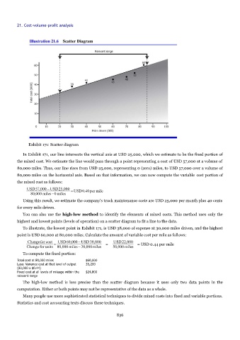
Exhibit 171: Scatter diagram

In Exhibit 171, our line intersects the vertical axis at USD 25,000, which we estimate to be the fixed portion of
the mixed cost. We estimate the line would pass through a point representing a cost of USD 57,000 at a volume of
80,000 miles. Thus, our line rises from USD 25,000, representing 0 (zero) miles, to USD 57,000 over a volume of

80,000 miles on the horizontal axis. Based on that information, we can now compute the variable cost portion of
the mixed cost as follows:
USD57,000 – USD25,000 =USD0.40per mile
80,000 miles –0 miles
Using this result, we estimate the company's truck maintenance costs are USD 25,000 per month plus 40 cents

for every mile driven.
You can also use the high-low method to identify the elements of mixed costs. This method uses only the
highest and lowest points (levels of operation) on a scatter diagram to fit a line to the data.
To illustrate, the lowest point in Exhibit 171, is USD 38,000 of expense at 30,000 miles driven, and the highest
point is USD 60,000 at 80,000 miles. Calculate the amount of variable cost per mile as follows:
Changefor cost USD60,000 – USD 38,000 USD22,000
=
Change for units 80,000 miles – 30,000miles = 50,000 miles = USD 0.44 per mile
To compute the fixed portion:
Total cost at 80,000 miles $60,000
Less: Variance cost at that level of output 35,200
(80,000 x $0.44)
Fixed cost at all levels of mileage within the $24,800
relevant range
The high-low method is less precise than the scatter diagram because it uses only two data points in the
computation. Either or both points may not be representative of the data as a whole.
Many people use more sophisticated statistical techniques to divide mixed costs into fixed and variable portions.
Statistics and cost accounting texts discuss these techniques.

836