Page 104 - Finanancial Management_2022

LOOKUP(lookup_value, array) LOOKUP in vector form with Helper

where:
• lookup_value is the value that
LOOKUP searches for in an array.
The lookup_value
argument can be a number, text, a
logical value, or a name or reference
that refers to a value.
• array is the range of cells that
contains text, numbers, or logical
values that you want to compare
with lookup_value.
The array form of LOOKUP is
very similar to the HLOOKUP and
VLOOKUP functions. The difference
is that HLOOKUP searches for the
value of lookup_value in the first row,
VLOOKUP searches in the first column,
and LOOKUP searches according to the
dimensions of array.
If the array covers an area that is
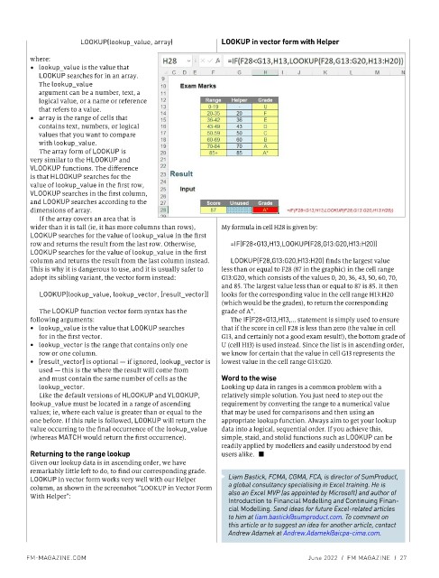
wider than it is tall (ie, it has more columns than rows), My formula in cell H28 is given by:
LOOKUP searches for the value of lookup_value in the first
row and returns the result from the last row. Otherwise, =IF(F28<G13,H13,LOOKUP(F28,G13:G20,H13:H20))
LOOKUP searches for the value of lookup_value in the first
column and returns the result from the last column instead. LOOKUP(F28,G13:G20,H13:H20) finds the largest value
This is why it is dangerous to use, and it is usually safer to less than or equal to F28 (87 in the graphic) in the cell range
adopt its sibling variant, the vector form instead: G13:G20, which consists of the values 0, 20, 36, 43, 50, 60, 70,
and 85. The largest value less than or equal to 87 is 85. It then
LOOKUP(lookup_value, lookup_vector, [result_vector]) looks for the corresponding value in the cell range H13:H20
(which would be the grades), to return the corresponding
The LOOKUP function vector form syntax has the grade of A*.
following arguments: The IF(F28<G13,H13,… statement is simply used to ensure
y lookup_value is the value that LOOKUP searches that if the score in cell F28 is less than zero (the value in cell
for in the first vector. G13, and certainly not a good exam result!), the bottom grade of
y lookup_vector is the range that contains only one U (cell H13) is used instead. Since the list is in ascending order,
row or one column. we know for certain that the value in cell G13 represents the
y [result_vector] is optional — if ignored, lookup_vector is lowest value in the cell range G13:G20.
used — this is the where the result will come from
and must contain the same number of cells as the Word to the wise
lookup_vector. Looking up data in ranges is a common problem with a
Like the default versions of HLOOKUP and VLOOKUP, relatively simple solution. You just need to step out the
lookup_value must be located in a range of ascending requirement by converting the range to a numerical value
values; ie, where each value is greater than or equal to the that may be used for comparisons and then using an
one before. If this rule is followed, LOOKUP will return the appropriate lookup function. Always aim to get your lookup
value occurring to the final occurrence of the lookup_value data into a logical, sequential order. If you achieve this,
(whereas MATCH would return the first occurrence). simple, staid, and stolid functions such as LOOKUP can be
readily applied by modellers and easily understood by end
Returning to the range lookup users alike. ■
Given our lookup data is in ascending order, we have
remarkably little left to do, to find our corresponding grade.
LOOKUP in vector form works very well with our Helper Liam Bastick, FCMA, CGMA, FCA, is director of SumProduct,
column, as shown in the screenshot “LOOKUP in Vector Form a global consultancy specialising in Excel training. He is
With Helper”: also an Excel MVP (as appointed by Microsoft) and author of
Introduction to Financial Modelling and Continuing Finan-
cial Modelling. Send ideas for future Excel-related articles
to him at liam.bastick@sumproduct.com. To comment on
this article or to suggest an idea for another article, contact
Andrew Adamek at Andrew.Adamek@aicpa-cima.com.

FM-MAGAZINE.COM June 2022 I FM MAGAZINE I 27