Page 103 - Finanancial Management_2022

LEARNING RESOURCE
Therefore, the formula:

=LEFT(F13,IFERROR(FIND("-",F13),FIND("+",F13))-1)
Advanced Excel: will return the text equivalent of the first number
Practical Applications for in the range for all buckets. For example, in row 20,
Accounting Professionals
IFERROR(FIND("-",F13),FIND("+",F13)) returns three (3),
This online video course will make so the formula resolves to:
you excel in Excel. It’s designed for
accountants, by an accountant, so =LEFT(F20, 3 – 1)
you’ll learn how to unlock all the
magic in your spreadsheets. Using which would return the two “left-most” characters in
live workbook files that you can edit
as you go, you’ll become a master the text string “85+”, ie, “85”. However, this would not
in topics such as advanced pivot be a numerical value, so multiplying by one (1) converts
tables, external data ranges, and these text strings into numerical values, hence the final
the IF function, and features such formula:
as process automation.
All of which will help you work =LEFT(F13,IFERROR(FIND("-
faster and smarter. ",F13),FIND("+",F13))-1)*1
Find this course in the AICPA Store
and in the CGMA Store. This has now addressed our first issue. We now have
a numerical register (a list of values in increasing order)
COURSE we may use to look up our students’ marks. I now need
to consider which function to use to look up the data.
As with all things in Excel, simplest is best. Yes, we
Not my longest calculation ever by any means, but it have VLOOKUP, HLOOKUP, INDEX MATCH, OFFSET
still needs explaining. It all centres on the FIND function: MATCH, SUMIF, SUMIFS, SUMPRODUCT, XLOOKUP,
et al., but whenever you have data in ascending order in
FIND("-",F13) a spreadsheet, your simplest, most reliable function to
use is nothing more than the extremely humble LOOKUP
This formula looks for the character position of the function.
hyphen ("-") in cell F13. In the text string “0-19” (the
contents of cell F13), the hyphen is clearly the second LOOKUP reminder
character in the text string, so FIND("-",F13) will return the LOOKUP has two forms: an array form and a vector form.
value two (2). Let me explain the jargon:
If there is no hyphen, the error message #VALUE! is • An array is a collection of cells consisting of at least
returned instead. Hence, we “wrap” this formula in an two rows and at least two columns.
IFERROR expression as follows: • A vector is a collection of cells across just one row
(row vector) or down just one column (column
IFERROR(FIND("-",F13),FIND("+",F13)) vector).
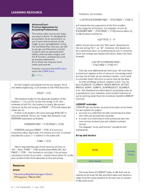
The diagram “Array and Vectors” should be self-
IFERROR evaluates FIND("-",F13). If it returns a explanatory.
numerical value, that’s fine; if it returns an error, it instead
searches for a plus (“+”) symbol in the same cell: Array and vectors

FIND("+",F13)

This is required because of the value in cell F20, ie,
“85+”. Here, FIND("-",F20) would return #VALUE!, but
FIND("+",F20) — the formula to calculate if the primary
calculation results in an error — would return three (3), as the
plus symbol is the third character in this text string.

Resources
Article
The array form of LOOKUP looks in the first row or
“ Calculating Weighted Averages in Excel”, column of an array for the specified value and returns a
FM magazine, 7 March 2022 value from the same position in the last row or column
of the same array:

26 I FM MAGAZINE I June 2022