Page 67 - Linear Models for the Prediction of Animal Breeding Values

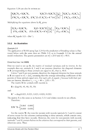
Equation 3.24 can also be written as:

′
⎡ X ′RX + X ′RX X ′R ZX RZ ⎤ ˆ ⎡ X R y − −1 ⎤
−1
−1
−1
−1
−1
1 ⎡ ⎤
+
b
n
n
⎥
⎢ p p p n n n p p n n 2 ⎢ ⎥ = ⎢ ′ p p p + X′ R y n ⎥
⎢ ⎣ ′ Z R X + 1 ′ Z RX n ′ Z R Z ZR Z 1 + A −1 1/s a ⎥ ⎦ a ⎣ ⎦ ˆ ⎢ ⎣ Z R y p +Z R y ⎥
′
−1
−1
− −1
−1
+ ′
−1
−1
′
n⎦
p
p
p
n
p
1
1
n
n
Multiplying the equations above by R gives:
p
1 ⎤
−
−
⎡ XX + n ′ − v 1 n X p ′Z XR Z 1 ⎡ ⎤ ˆ ⎡ X y ′ p p + XR y n ⎤
⎤
n ′
p ′
1
+
p X R X
b
v
′ n
v
⎢ − 1 − 1 −1 1 ⎥ ⎢ ⎥ = ⎢ − 1 ⎥ (3.25)
+
a ˆ
⎣ ⎢ ′ Z X + ′ 1 v n ′ ZZ Z RZ + A a ⎣ ⎦ ⎢ ⎣ Zy ′ p +Z R y n⎥ ⎦
⎦ ⎥
p Z RX
′ 1
′ 1
v
1
v
−1
−1
where R equals 1/(1 + Da ).
v
3.5.2 An illustration
Example 3.3
The application of RAM using Eqn 3.24 for the prediction of breeding values is illus-
trated below with the same data set (Table 3.1) as in Example 3.1 for the animal
2
2
model evaluation. The genetic parameters are s = 20.0 and s = 40.0.
a e
CONSTRUCTING THE MME
First we need to set up R, the matrix of residual variances and its inverse. In the
example data set, animals 4, 5 and 6 are parents; therefore the diagonal elements
2
in R corresponding to these animals are equal to s , that is, 40.0.
e
Calves 7 and 8 are non-parents, therefore the diagonal elements for these animals
in R are equal to s + d s , assuming that the average inbreeding coefficients of the
2
2
e i a
parents of these animals equal zero. For each calf, d equals because both their par-
1
i
2
1
ents are known, therefore r = r = 40 + 2 (20) = 50.
77 88
The matrix R for animals with records is:
R = diag(40, 40, 40, 50, 50)
and:
−1
R = diag(0.025, 0.025, 0.025, 0.020, 0.020)
The matrix X is the same as in Section 3.3.1 and relates records to sex effects.
Therefore:
⎡0.065 0.000 ⎤
′
−1
XR X = ⎢ ⎥
⎣ 0.000 0.050 ⎦
For the matrix W, the rows for parents with records (animals 4, 5 and 6) consist
of zeros except for the columns corresponding to these animals, which contain ones,
indicating that they have records. However, the rows for non-parents with records
(animals 7 and 8) contain halves in the columns that correspond to their parents, and
otherwise zeros. Thus:
Univariate Models with One Random Effect 51