Page 69 - Linear Models for the Prediction of Animal Breeding Values

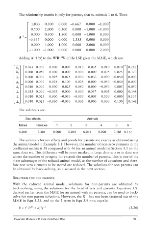
The relationship matrix is only for parents, that is, animals 1 to 6. Thus:

⎡ 1.833 0.500 0.000 −0.667 0.000 −1.000⎤
⎢ − ⎥
⎢ 0.500 2.000 0.500 0.000 −1.000 −1.000 ⎥
⎢ 0.000 0.500 1.500 0.000 −1.000 0.000⎥
A = ⎢ ⎥
−1
⎢ −0.667 0.000 0.0000 1.333 0.000 0.000 ⎥
⎢ 0.000 − 1.000 − 1.000 0.000 2.000 0.000 ⎥
⎢ ⎥
⎣ ⎢ − 1.000 − 1..000 0.000 0.000 0.000 2.000⎥ ⎦

−1
−1
2
Adding A 1/s to the W′R W of the LSE gives the MME, which are:
a
−1
⎡ b ⎤ ⎡ 0.0665 0.000 0.000 0.000 0.010 0.035 0.010 0.010⎤ ⎡0.282⎤
ˆ
⎢ ˆ ⎥ ⎢ ⎥ ⎥ ⎢ ⎥
1
⎢ b 2 ⎥ ⎢ 0.000 0.050 0.000 0.000 00.000 0.000 0.025 0.025 ⎥ ⎢ 0.170 ⎥
⎢ ⎥ ⎢ 0.000 0.000 0.092 0.025 0.000 − 0.033 0.000 −00.050⎥ ⎢0.000⎥
⎢ a ˆ 1 ⎥ ⎢ ⎥ ⎢ ⎥
⎢ a ˆ 2⎥ ⎢ 0.000 0.000 0.025 0.100 0.025 0.000 − 0.050 − 0.050 ⎥ ⎢ ⎢ 0.000 ⎥
=
⎢ a ˆ ⎥ ⎢ 0.010 0.000 0 0.000 0.025 0.080 0.000 − 0.050 0.005 ⎥ ⎢ 0.050 ⎥
⎢ 3 ⎥ ⎢ ⎥ ⎢ ⎥
⎢ a ˆ 4⎥ ⎢ 0.035 0.000 − 0.033 0.000 0.000 0 0.097 0.005 0.000⎥ ⎢ 0.148⎥
⎢ ⎥ ⎢ 0.000 − 0.050 − ⎥ ⎢ ⎥
⎢ a ˆ 5 ⎥ ⎢ 0.010 0.025 0.050 0.005 0.130 0.000 ⎥ ⎢ 0.107 ⎥
⎢ ⎣ a ˆ 6⎦ ⎣ 0 0.010 0.025 − 0.050 − 0.050 0.005 0.000 0.000 0.130⎥ ⎢ 0.148⎥ ⎦
⎥ ⎢
⎦ ⎣
The solutions are:
Sex effects Animals
Males Females 1 2 3 4 5 6
4.358 3.404 0.098 −0.019 −0.041 −0.009 −0.186 0.177

The solutions for sex effects and proofs for parents are exactly as obtained using
the animal model in Example 3.1. However, the number of non-zero elements in the
coefficient matrix is 38 compared with 46 for an animal model in Section 3.3 on the
same data set. This difference will be more marked in large data sets or in data sets
where the number of progeny far exceeds the number of parents. This is one of the
main advantages of the reduced animal model, as the number of equations and there-
fore non-zero elements to be stored are reduced. The solutions for non-parents can
be obtained by back-solving, as discussed in the next section.

SOLUTIONS FOR NON-PARENTS
With the reduced animal model, solutions for non-parents are obtained by
back-solving, using the solutions for the fixed effects and parents. Equation 3.9,
derived earlier from the MME for an animal with its parents, can be used to back-
−1
solve for non-parent solutions. However, the R has not been factored out of the
MME in Eqn 3.25, and so the k term in Eqn 3.9 now equals:
k = r /r + d g (3.26)
11
−1 −1
11
i
Univariate Models with One Random Effect 53