Page 72 - Linear Models for the Prediction of Animal Breeding Values

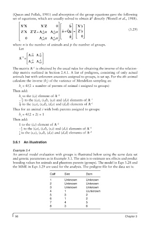
(Quaas and Pollak, 1981) and absorption of the group equations gave the following
ˆ
set of equations, which are usually solved to obtain a* directly (Westell et al., 1988).
⎡ ⎤ ˆ ⎤
′
′
⎢ XX XZ 0 ⎡ ⎢ b ⎥ ⎡ Xy ′ ⎤
⎥
⎢ ′ −1 A a ⎢ aQg = ⎢ Zy ′ ⎥ (3.29)
ˆ
⎥ ˆ
+
⎥
g
−1
′ +
⎢ ZX ZZ A a np ⎥ ⎢ ⎥ ⎢ ⎥
nn
⎢ −1 A a ⎣ g ˆ ⎦ ⎢ ⎣ 0⎥ ⎦
⎥
−1
⎣ 0 A a pp ⎦
pn
where n is the number of animals and p the number of groups.
Let
⎡ A nn A np ⎤
−1
−1
A = ⎢ ⎥
−1
⎢ ⎣ A pn A pp ⎥ ⎦
−1
−1
−1
The matrix A is obtained by the usual rules for obtaining the inverse of the relation-
ship matrix outlined in Section 2.4.1. A list of pedigrees, consisting of only actual
animals but with unknown ancestors assigned to groups, is set up. For the ith animal
calculate the inverse (b ) of the variance of Mendelian sampling as:
i
b = 4/(2 + number of parents of animal i assigned to groups)
i
Then add:
b to the (i,i) element of A −1
i
− to the (i,s), (i,d), (s,i) and (d,i) elements of A −1
b i
2
b i to the (s,s), (s,d), (d,s) and (d,d) elements of A −1
4
Thus for an animal i with both parents assigned to groups:
b = 4/(2 + 2) = 1
i
Then add:
1 to the (i,i) element of A −1
1
− to the (i,s), (i,d), (s,i) and (d,i) elements of A −1
2
1 to the (s,s), (s,d), (d,s) and (d,d) elements of A −1
4
3.6.1 An illustration
Example 3.4
An animal model evaluation with groups is illustrated below using the same data set
and genetic parameters as in Example 3.1. The aim is to estimate sex effects and predict
breeding values for animals and phantom parents (groups). The model in Eqn 3.28 and
the MME in Eqn 3.29 are used for the analysis. The pedigree file for the data set is:
Calf Sire Dam
1 Unknown Unknown
2 Unknown Unknown
3 Unknown Unknown
4 1 Uunknown
5 3 2
6 1 2
7 4 5
8 3 6
56 Chapter 3