Page 75 - Linear Models for the Prediction of Animal Breeding Values

The animal proofs above are generally lower than those from Example 3.1, the
model without groups. In addition, the ranking for animals is also different. However,
the relationship between the two sets of solutions can be shown by recalculating the
ˆ
vector of solutions for animals using the group solutions (g) above and the estimated
ˆ
breeding values (a) from Example 3.1 as:
a = aˆ + Qg
ˆ
*
where Q = TQ * , as defined earlier.
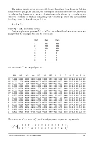
Assigning phantom parents (M1 to M7) to animals with unknown ancestors, the
pedigree for the example data can be written as:

Calf Sire Dam
1 M1 M2
2 M3 M4
3 M5 M6
4 1 M7
5 3 2
6 1 2
7 4 5
8 3 6

and the matrix T for the pedigree is:

M1 M2 M3 M4 M5 M6 M7 1 2 3 4 5 6 7 8
M1 1.000 0.000 0.000 0.000 0.000 0.000 0.00 0.00 0.00 0.00 0.0 0.0 0.0 0.0 0.0
M2 0.000 1.000 0.000 0.000 0.000 0.000 0.00 0.00 0.00 0.00 0.0 0.0 0.0 0.0 0.0
M3 0.000 0.000 1.000 0.000 0.000 0.000 0.00 0.00 0.00 0.00 0.0 0.0 0.0 0.0 0.0
M4 0.000 0.000 0.000 1.000 0.000 0.000 0.00 0.00 0.00 0.00 0.0 0.0 0.0 0.0 0.0
M5 0.000 0.000 0.000 0.000 1.000 0.000 0.00 0.00 0.00 0.00 0.0 0.0 0.0 0.0 0.0
M6 0.000 0.000 0.000 0.000 0.000 1.000 0.00 0.00 0.00 0.00 0.0 0.0 0.0 0.0 0.0
M7 0.000 0.000 0.000 0.000 0.000 0.000 1.00 0.00 0.00 0.00 0.0 0.0 0.0 0.0 0.0
1 0.500 0.500 0.000 0.000 0.000 0.000 0.00 1.00 0.00 0.00 0.0 0.0 0.0 0.0 0.0
2 0.000 0.000 0.500 0.500 0.000 0.000 0.00 0.00 1.00 0.00 0.0 0.0 0.0 0.0 0.0
3 0.000 0.000 0.000 0.000 0.500 0.500 0.00 0.00 0.00 1.00 0.0 0.0 0.0 0.0 0.0
4 0.250 0.250 0.000 0.000 0.000 0.000 0.50 0.50 0.00 0.00 1.0 0.0 0.0 0.0 0.0
5 0.000 0.000 0.250 0.250 0.250 0.250 0.00 0.00 0.50 0.50 0.0 1.0 0.0 0.0 0.0
6 0.250 0.250 0.250 0.250 0.000 0.000 0.00 0.50 0.50 0.00 0.0 0.0 1.0 0.0 0.0
7 0.125 0.125 0.125 0.125 0.125 0.125 0.25 0.25 0.25 0.25 0.5 0.5 0.0 1.0 0.0
8 0.125 0.125 0.125 0.125 0.250 0.250 0.00 0.25 0.25 0.50 0.0 0.0 0.5 0.0 1.0

The transpose of the matrix Q * , which assigns phantom parents to groups is:

⎛1 0 1 0 1 0 0 0 0 0 0 0 0 0 0 ⎞
Q ′ = ⎜ ⎟
*
⎝0 1 0 1 0 1 0 0 0 0 0 0 0 0 0 ⎠

Univariate Models with One Random Effect 59