Page 70 - Linear Models for the Prediction of Animal Breeding Values

Solutions for non-parents in Example 3.3 can be solved using Eqn 3.9 but with k
expressed as in Eqn 3.26. However, because there is a fixed effect in the model, m =
i
k(y − b − 0.5a − 0.5a ). In Example 3.3, both parents of non-parents (animals 7 and 8)
c j s d
are known, therefore:
k = 0.025/(0.025 + (2)0.05) = 0.20
Solution for calves 7 and 8 are:
ˆ
a = 0.5(−0.009 + −0.186) + 0.20(3.5 − 4.358 − 0.5(−0.009 + −0.186))
7
= −0.249
a = 0.5(−0.041 + 0.177) + 0.20(5.0 −4.358 − 0.5(−0.041 + 0.177))
ˆ
8
= 0.183
Again, these solutions are the same for these animals as under the animal model.
3.5.3 An alternative approach

Note that, if the example data had been analysed using Eqn 3.25, the design matrices
would be of the following form:
⎡ 10 0⎤ ⎡ 11⎤
X′ = ⎢ ⎥ , X′ = ⎢ ⎥
n
p
⎣ 01 1 ⎦ ⎣ 00 ⎦
Z including ancestors is:
⎡ 000 1 0 0⎤
⎢ ⎥ ⎡ 00 0 0.5 0.5 0 ⎤
=
Z = ⎢ 0000 1 0 ⎥ and Z1 ⎢ ⎥
⎢ ⎣ 00000 1⎥ ⎦ ⎣ 000.5 0 0 0..5 ⎦
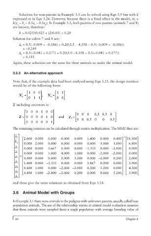
The remaining matrices can be calculated through matrix multiplication. The MME then are:

ˆ ⎡ ⎤
1 b
−1
⎢ ⎥ ⎡ 2.600 0.000 0.000 0.000 0.400 1.400 0.400 0.400⎤ ⎡ 11.300⎤
b ⎢ ˆ 2⎥ ⎢ ⎥ ⎢ ⎥
⎢ ⎥ ⎢ 0.000 2.000 0.0000 0.000 0.000 0.000 1.000 1.000 ⎥ ⎢ 6.800 ⎥
1 ˆ a
⎢ ⎥ ⎢ 0.000 0.000 3.667 1.000 0.000 − 1.333 0.000 − 2.000⎥ ⎢ 0.000⎥
3
1 ˆ a ⎢ ⎥ ⎢ ⎥ ⎢ ⎥
⎢ ⎥ ⎢ 0.000 0.000 1.000 4.000 1.000 0.000 − 2.000 − 2.000 ⎥ ⎢ 0.000 ⎥
= =
2 ˆ a
⎢ ⎥ ⎢ 0.4000 0.000 0.000 1.000 3.200 0.000 − 2.000 0.200 ⎥ ⎢ 2.000 ⎥
⎢ ⎥ ⎢ ⎢ ⎥ ⎢ ⎥
3 ˆ a
⎢ ⎥ ⎢ 1.400 0.000 − 1.333 0.0000 0.000 3.867 0.200 0.000⎥ ⎢ 5.900⎥
4 ˆ a ⎢ ⎥ ⎢ 0.000 − 2.000 − ⎥ ⎢ ⎥
⎢ ⎥ ⎢ 0.400 1.000 2.000 0.200 5.2000 0.000 ⎥ ⎢ 4.300 ⎥
4 ˆ a
⎢ ⎥ ⎢ ⎣ 0.400 1.000 − 2.000 − 2.000 0.200 0.000 0.000 5.200⎥ ⎢ 5.9000⎥ ⎦
⎦ ⎣
6 ˆ a ⎣ ⎢ ⎦ ⎥
and these give the same solutions as obtained from Eqn 3.24.
3.6 Animal Model with Groups
In Example 3.1 there were animals in the pedigree with unknown parents, usually called base
population animals. The use of the relationship matrix in animal model evaluation assumes
that these animals were sampled from a single population with average breeding value of

54 Chapter 3