Page 74 - Linear Models for the Prediction of Animal Breeding Values 3rd Edition

−1
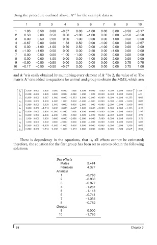
Using the procedure outlined above, A for the example data is:
1 2 3 4 5 6 7 8 9 10

1 1.83 0.50 0.00 −0.67 0.00 −1.00 0.00 0.00 −0.50 −0.17
2 0.50 2.00 0.50 0.00 −1.00 −1.00 0.00 0.00 −0.50 −0.50
3 0.00 0.50 2.00 0.00 −1.00 0.50 0.00 −1.00 −0.50 −0.50
4 −0.67 0.00 0.00 1.83 0.50 0.00 −1.00 0.00 0.00 −0.67
5 0.00 −1.00 −1.00 0.50 2.50 0.00 −1.00 0.00 0.00 0.00
6 −1.00 −1.00 0.50 0.00 0.00 2.50 0.00 −1.00 0.00 0.00
7 0.00 0.00 0.00 −1.00 −1.00 0.00 2.00 0.00 0.00 0.00
8 0.00 0.00 −1.00 0.00 0.00 −1.00 0.00 2.00 0.00 0.00
9 −0.50 −0.50 −0.50 0.00 0.00 0.00 0.00 0.00 0.75 0.75
10 −0.17 −0.50 −0.50 −0.67 0.00 0.00 0.00 0.00 0.75 1.08

−1
and A a is easily obtained by multiplying every element of A by 2, the value of a. The
−1
−1
matrix A a is added to equations for animal and group to obtain the MME, which are:
⎡ b 1 ⎤ ⎡ 3.000 0.000 0.000 0.000 0.000 1.000 0.000 0 0.000 1.000 1.000 0.000 0.000⎤ −1 ⎡ 13.0 ⎤
ˆ
⎢ ˆ ⎥ ⎥ ⎢ ⎥ ⎢ ⎥
⎢ b 2 ⎥ ⎢ 0.000 2.000 0.000 0.000 0.000 0.000 1..000 1.000 0.000 0.000 0.000 0.000 ⎥ ⎥ ⎢ 6.8 ⎥
⎢ a ˆ 1 ⎥ ⎢ 0.000 0.000 3.667 1.000 0.000 − 1.3333 0.000 − 2.000 0.000 0.000 − 1.000 − 0.333 ⎥ ⎢ 0.00 ⎥
⎢ ⎥ ⎢ ⎥ ⎢ ⎥
⎢ a ˆ 2⎥ ⎢ 0.000 0.000 1.000 4.000 1..000 0.000 − 2.000 − 2.000 0.000 0.000 − 1.000 − 1.000 ⎥ ⎢ 0.00 ⎥
⎢ ⎥ ⎢ 0.000 0.000 0.000 0 1.000 4.000 0.000 − 2.000 1.000 0.000 − 2.000 − 1.000 − 1.000 ⎥ ⎢ 0.00 ⎥
⎢ a ˆ 3 ⎥ ⎢ ⎥ ⎢ ⎥
⎢ a ˆ 4 ⎥ ⎢ 1.000 0.0000 − 1.333 0.000 0.000 4.667 1.000 0.000 − 2.000 0.000 0.000 − 1.333⎥ ⎢ 4.50 ⎥
⎢ ⎥ = ⎢ ⎥ ⎢ ⎥
⎢ a ˆ 5 ⎥ ⎢ 0..000 1.000 0.000 − 2.000 − 2.000 1.000 6.000 0.000 − 2.000 0.000 0.000 0 0.000 ⎥ ⎢ 2.90 ⎥
⎢ ⎥ ⎢ 0.000 1.000 − 2.000 − 2.000 1.000 0.000 0.000 6.000 0.000 − 2.000 0 0.000 0.000 ⎥ ⎢ 3.90 ⎥
⎢ a ˆ 6 ⎥ ⎢ ⎥ ⎢ ⎥
⎢ a ˆ 7 ⎥ ⎢ 1.000 0.000 0.000 0.000 0.000 − 2.000 − 2.000 0.000 5.000 0 0.000 0.000 0.000⎥ ⎢ 3.50 ⎥
⎢ ⎥ ⎢ ⎥ ⎢ ⎥
⎢ a ˆ 8 ⎥ ⎢ 1.000 0.000 0.000 0.000 − 2.000 0.000 0.000 − 2.000 0 0.000 5.000 0.000 0.000 ⎥ ⎢ 5.00 ⎥
⎢ 1 ˆ g ⎥ ⎢ 0.000 0.000 − 1.000 − 1.000 − 1.000 0.000 0.0000 0.000 0.000 0.000 1.500 1.500 ⎥ ⎢ 0 0.00 ⎥
⎢ ⎥ ⎢ ⎥ ⎢ ⎥
⎣ ⎢ g ˆ ⎥ ⎣ ⎢ 0.000 0.000 − 0.333 − 1.000 − 1.000 − 1..333 0.000 0.000 0.000 0.000 1.500 2.167 ⎦ ⎥ ⎣ ⎢ 0.00 ⎦ ⎥
2⎦
There is dependency in the equations, that is, all effects cannot be estimated;
therefore, the equation for the first group has been set to zero to obtain the following
solutions:
Sex effects
Males 5.474
Females 4.327
Animals
1 −0.780
2 −0.936
3 −0.977
4 −1.287
5 −1.113
6 −0.741
7 −1.354
8 −0.782
Groups
9 0.000
10 −1.795

58 Chapter 3