Page 76 - Linear Models for the Prediction of Animal Breeding Values 3rd Edition

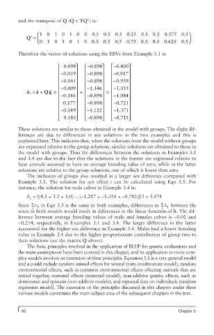
and the transpose of Q (Q = TQ * ) is:

⎛ 1 0 1 0 1 0 0 0.5 0.5 0.5 0.25 0.5 0.5 0.375 0.5⎞
Q ′ = ⎜ ⎝ 0 1 0 1 0 1 0 0.5 0.5 0.5 0.75 00.5 0.5 0.625 0.5⎠ ⎟

Therefore the vector of solutions using the EBVs from Example 3.1 is:

⎡ 0.098⎤ ⎡ − 0.898⎤ ⎡ −0.8000⎤ ⎤
⎢ − ⎥ ⎢ − ⎥ ⎢ − ⎥
⎢ 0.019 ⎥ ⎢ 0.898 ⎥ ⎢ 0.917 ⎥
⎢ − 0.041⎥ ⎢ − 0.898⎥ ⎢ − 0.939⎥
⎢ − ⎥ ⎢ − ⎥ ⎢ − ⎥
ˆ a = ˆ a + Q ˆ g = ⎢ 0.009 ⎥ + ⎢ 1.346 ⎥ = ⎢ 1.355 ⎥
* ⎢ − 0.186 ⎥ ⎢ − −0.898 ⎥ ⎢ − 1.084 ⎥
⎢ ⎥ ⎢ ⎥ ⎢ ⎥
⎢ 0.177 ⎥ ⎢ −0.898 ⎥ ⎢ − 0.721 ⎥
⎢ − ⎥ ⎢ ⎥ ⎢ − ⎥
⎢ 0.249 ⎥ ⎢ −1.122 ⎥ ⎢ 1.371 ⎥
⎣ ⎢ 0..183⎥ ⎦ ⎣ ⎢ −0.898⎥ ⎦ ⎣ ⎢ − 0.715⎥ ⎦

These solutions are similar to those obtained in the model with groups. The slight dif-
ferences are due to differences in sex solutions in the two examples and this is
explained later. This indicates that, when the solutions from the model without groups
are expressed relative to the group solutions, similar solutions are obtained to those in
the model with groups. Thus the differences between the solutions in Examples 3.1
and 3.4 are due to the fact that the solutions in the former are expressed relative to
base animals assumed to have an average breeding value of zero, while in the latter
solutions are relative to the group solutions, one of which is lower than zero.
The inclusion of groups also resulted in a larger sex difference compared with
Example 3.1. The solution for sex effect i can be calculated using Eqn 3.5. For
instance, the solution for male calves in Example 3.4 is:
b = [(4.5 + 3.5 + 5.0) − (−1.287 + −1.354 + −0.782)]/3 = 5.474
1
Since å y in Eqn 3.5 is the same in both examples, differences in ∑ a between the
ˆ
j ij j ij
sexes in both models would result in differences in the linear function of b. The dif-
ference between average breeding values of male and females calves is −0.02 and
−0.214, respectively, in Examples 3.1 and 3.4. The larger difference in the latter
accounted for the higher sex difference in Example 3.4. Males had a lower breeding
value in Example 3.4 due to the higher proportionate contribution of group two to
their solutions (see the matrix Q above).
The basic principles involved in the application of BLUP for genetic evaluations and
the main assumptions have been covered in this chapter, and its application to more com-
plex models involves an extension of these principles. Equation 3.1 is a very general model
and a could include random animal effects for several traits (multivariate model), random
environmental effects, such as common environmental effects affecting animals that are
reared together, maternal effects (maternal model), non-additive genetic effects, such as
dominance and epistasis (non-additive models), and repeated data on individuals (random
regression model). The extension of the principles discussed in this chapter under these
various models constitutes the main subject area of the subsequent chapters in the text.

60 Chapter 3