Page 80 - Linear Models for the Prediction of Animal Breeding Values 3rd Edition

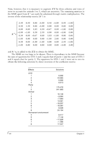
Note, however, that it is necessary to augment Z′Z by three columns and rows of
zeros to account for animals 1 to 3, which are ancestors. The remaining matrices in
−1
the MME apart from A can easily be calculated through matrix multiplication. The
−1
inverse of the relationship matrix (A ) is:
⎡ 2.50 0.50 0.00 –1.00 0.50 –1.00 0.50 –1.00⎤
⎢ ⎥
⎢ 0.50 1.50 0.00 –1.00 0 0.00 0.00 0.00 0.00 ⎥
⎢ 0.00 0.00 1.83 0.50 –0.67 0.00 –1.00 0.00⎥
⎢ ⎥
–1 ⎢ ⎢ –1.00 –1..00 0.50 2.50 0.00 0.00 –1.00 0.00 ⎥
A = ⎢ ⎥
0
⎢ 0.50 0.00 –0.67 0.00 1.83 –1.00 0.00 0.00 ⎥
⎢ –1.00 0.00 0.00 0.00 –1.00 2.00 0.00 0.00 ⎥
⎢ 0.50 0.00 –1.00 –1.00 0 0.00 0.00 2.50 –1.00 ⎥
⎢ ⎥
⎣ ⎢ –1.00 0.00 0.00 0.00 0.00 0.00 –1.00 2.00⎥ ⎦

−1
and A a is added to the Z′Z to obtain the MME.
1
The MME are too large to be shown. There is dependency in the MME because
the sum of equations for HYS 1 and 2 equals that of parity 1 and the sum of HYS 3
and 4 equals that for parity 2. The equations for HYS 1 and 3 were set to zero to
obtain the following solutions by direct inversion of the coefficient matrix:

Effects Solutions
HYS
1 0.000
2 44.065
3 0.000
4 0.013
Parity
1 175.472
2 241.893
Animal
1 10.148
2 −3.084
3 −7.063
4 13.581
5 −18.207
6 −18.387
7 9.328
8 24.194
Permanent environment
4 8.417
5 −7.146
6 −17.229
7 −1.390
8 17.347

64 Chapter 4