Page 82 - Linear Models for the Prediction of Animal Breeding Values 3rd Edition

favourable – for instance, animal 8 has the highest estimates of pe and this is reflected
by her high average yield – or could reduce performance (for example, cow 6 has a
very negative estimate of pe and low average yield). A practical example of such per-
manent environment effect could be the loss of a teat by a cow early in life due to
infection. Thus differences in estimates of pe represent permanent environmental dif-
ferences between animals and could help the farmer, in addition to the breeding value,
in selecting animals for future performance in the same herd. The sum of breeding
ˆ
value and permanent environment effect (a + pe ) for animal i is termed the probable
i i
producing ability (PPA) and represents an estimate of the future performance of the
animal in the same herd. If the estimate of the management level (M) for animal i is
known, its future record (y ) can be predicted as:
i
y = M + PPA
i
This could be used as a culling guide.

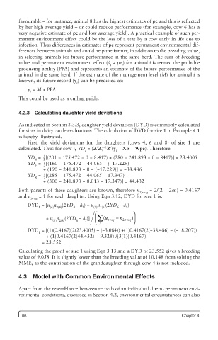
4.2.3 Calculating daughter yield deviations

As indicated in Section 3.3.3, daughter yield deviation (DYD) is commonly calculated
for sires in dairy cattle evaluations. The calculation of DYD for sire 1 in Example 4.1
is hereby illustrated.
First, the yield deviations for the daughters (cows 4, 6 and 8) of sire 1 are
−1
calculated. Thus for cow i, YD = (Z′Z) Z′(y − Xb − Wpe). Therefore:
i i
1
YD = [(201 − 175.472 − 0 − 8.417) + (280 − 241.893 − 0 − 8417)] = 23.4005
4 2
YD = 1 [(160 − 175.472 − 44.065 − (−17.229))
6 2
+ (190 − 241.893 − 0 − (−17.229)] = −38.486
YD = [(285 − 175.472 − 44.065 − 17.347)
1
8 2
+ (300 − 241.893 − 0.013 − 17.347)] = 44.432
Both parents of these daughters are known, therefore n = 2/(2 + 2a ) = 0.4167
2prog 1
and u = 1 for each daughter. Using Eqn 3.12, DYD for sire 1 is:
prog
ˆ
DYD = [u n (2YD - a ) + u n (2YD - a )
ˆ
1 (4) 2(4) 4 2 (5) 2(6) 6 5
⎛ ⎞
)
+ u n (2YD - a )] ⎜∑ (u prog + n 2 prog ⎟
ˆ
(8) 2(8) 8 7 ⎝ 3 ⎠
DYD = [(1)(0.4167)(2(23.4005) − (−3.084)) +(1)0.4167(2(−38.486) − (−18.207))
1
+ (1)0.4167(2(44.432) − 9.328)]/(3(1)(0.4167))
= 23.552
Calculating the proof of sire 1 using Eqn 3.13 and a DYD of 23.552 gives a breeding
value of 9.058. It is slightly lower than the breeding value of 10.148 from solving the
MME, as the contribution of the granddaughter through cow 4 is not included.
4.3 Model with Common Environmental Effects
Apart from the resemblance between records of an individual due to permanent envi-
ronmental conditions, discussed in Section 4.2, environmental circumstances can also

66 Chapter 4