Page 87 - Linear Models for the Prediction of Animal Breeding Values 3rd Edition

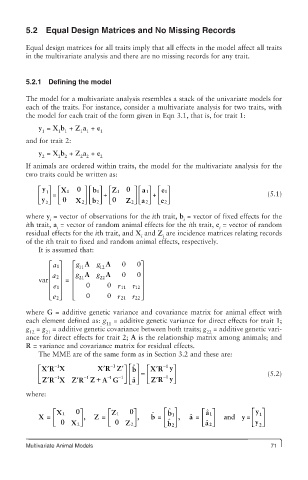
5.2 Equal Design Matrices and No Missing Records

Equal design matrices for all traits imply that all effects in the model affect all traits
in the multivariate analysis and there are no missing records for any trait.

5.2.1 Defining the model

The model for a multivariate analysis resembles a stack of the univariate models for
each of the traits. For instance, consider a multivariate analysis for two traits, with
the model for each trait of the form given in Eqn 3.1, that is, for trait 1:

y = X b + Z a + e
1 1 1 1 1 1
and for trait 2:
y = X b + Z a + e
2 2 2 2 2 2
If animals are ordered within traits, the model for the multivariate analysis for the
two traits could be written as:
⎡ y ⎤ ⎡ X 1 0 ⎤ ⎡ 1 b ⎤ ⎡ Z 1 0 ⎤ ⎡ 1 a ⎤ ⎡ ⎤
e1
1
+
=
⎢ ⎥ ⎢ ⎥ ⎢ ⎥ ⎢ ⎥ ⎢ ⎢ ⎥ ⎢ ⎥ (5.1)
+
⎣ y 2⎦ ⎣ 0 X 2⎦ ⎣ 2 b ⎦ ⎣ 0 Z 2⎦ ⎣ 2 a ⎦ ⎣ ⎦
e 2
where y = vector of observations for the ith trait, b = vector of fixed effects for the
i i
ith trait, a = vector of random animal effects for the ith trait, e = vector of random
i i
residual effects for the ith trait, and X and Z are incidence matrices relating records
i i
of the ith trait to fixed and random animal effects, respectively.
It is assumed that:
⎡ 1 a ⎤ ⎡ g A g A 0 0⎤
12
11
⎢ ⎥ ⎢ g A g A 0 0 ⎥
var ⎢ 2 a ⎥ = ⎢ 21 22 ⎥
⎢ 1 e ⎥ ⎢ 0 0 r 11 r ⎥
⎢ ⎥ ⎢ 12 ⎥
2 e ⎣ ⎦ ⎣ 0 0 r 2 21 r ⎦
22
where G = additive genetic variance and covariance matrix for animal effect with
each element defined as: g = additive genetic variance for direct effects for trait 1;
11
g = g = additive genetic covariance between both traits; g = additive genetic vari-
12 21 22
ance for direct effects for trait 2; A is the relationship matrix among animals; and
R = variance and covariance matrix for residual effects.
The MME are of the same form as in Section 3.2 and these are:
⎡ X R X X R Z′⎤ ⎡ ⎤ ˆ b ⎡ X R y⎤
′
−1
′
−1
′
−1
⎢ −1 −1 1 − −1 ⎥ ⎢ ⎥ = ⎢ −1 ⎥ (5.2)
′
′
⎣ Z R X Z R Z + A G ⎦ ⎣ ⎢ ⎦ ⎥ ˆ a ⎣ Z′′R y ⎦
where:
⎡ X1 0⎤ ⎡ Z1 0⎤ ⎡ ˆ ⎤ 1 a ˆ ⎡ ⎤ y ⎡ ⎤
=
X = ⎢ ⎥ , Z = ⎢ ⎥ , b ˆ = ⎢ b1 ⎥ , a ˆ = ⎢ ⎥ and y = ⎢ 1 ⎥
ˆ
⎣ 0 X 2⎦ ⎣ 0 Z2⎦ ⎣ b 2⎦ 2 a ˆ ⎣ ⎦ ⎣ y 2⎦
Multivariate Animal Models 71