Page 89 - Linear Models for the Prediction of Animal Breeding Values 3rd Edition

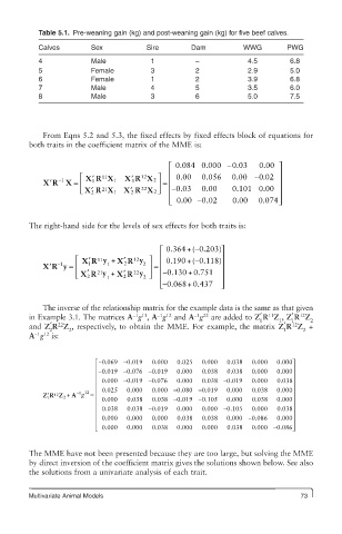
Table 5.1. Pre-weaning gain (kg) and post-weaning gain (kg) for five beef calves.
Calves Sex Sire Dam WWG PWG
4 Male 1 – 4.5 6.8
5 Female 3 2 2.9 5.0
6 Female 1 2 3.9 6.8
7 Male 4 5 3.5 6.0
8 Male 3 6 5.0 7.5

From Eqns 5.2 and 5.3, the fixed effects by fixed effects block of equations for
both traits in the coefficient matrix of the MME is:

⎡ ⎢ 0.084 0.0000 − 0.03 0.00 ⎤ ⎥
′
12
11
XR X = ⎡ XR X 1 X 1 ′ R X 2 ⎤ ⎥ = ⎢ 0.00 0.056 0.00 − 0.02 ⎥
′
−1
1
⎢
21
22
⎣ XR X 1 X 2 ′ R X 2 ⎦ − ⎢ 0.03 0.00 0.101 0.00 ⎥
′ 2
⎢ ⎥
⎣ 0.00 − 0.02 0 0.00 0.074 ⎦
The right-hand side for the levels of sex effects for both traits is:
−
⎡ 0 0.364 + ( 0.203)⎤
′
′
−
⎡ XR y + XR y ⎤ ⎢ 0.190 + ( 0.118) ⎥
11
12
XR y = ⎢ 1 1 2 ⎥ = ⎢ ⎥
2
′
−1
′
′
⎣ ⎢ XR y + XR y 2 ⎦ ⎥ ⎢ − ⎢ 0.130 + 0.751 ⎥ ⎥
22
21
2
2
1
⎣ − 0.068 + 0.4437 ⎦
The inverse of the relationship matrix for the example data is the same as that given
−1 22
11
12
−1 12
−1 11
in Example 3.1. The matrices A g , A g and A g are added to Z ′ R Z , Z ′ R Z
1 1 1 2
12
22
and Z ′ R Z , respectively, to obtain the MME. For example, the matrix Z ′ R Z +
2 2 1 2
−1 12
A g is:
⎡ −0.069 −0.019 0.000 0.025 0.000 0.038 0.000 0.0000⎤
⎢ − 0.019 − 0.076 − ⎥
⎢ 0.019 0.000 0.038 0.038 0.000 0.000 ⎥
⎢ 0.000 − 0.019 −00.076 0.000 0.038 − 0.019 0.000 0.038⎥
⎢ 0.025 0.000 0.000 − 0.080 − 0.019 9 0.000 0.038 0.000 ⎥
−
1 12
′
+
ZR 12 Z 2 A g = ⎢ ⎢ 0.038 − 0.019 − ⎥ ⎥
1
0
⎢ 0.000 0.038 0.105 0.000 0.038 0.000 ⎥
⎢ 0.038 0.038 − 0.019 0.000 0.000 − 0.105 0.000 0.038⎥
⎢ 0.000 − ⎥
⎢ 0.000 0.000 0.000 0 0.038 0.038 0.086 0.000 ⎥
⎢ ⎣ 0.000 0.000 0.038 0.000 0.000 0.038 0 0.000 − 0.086 ⎦ ⎥
The MME have not been presented because they are too large, but solving the MME
by direct inversion of the coefficient matrix gives the solutions shown below. See also
the solutions from a univariate analysis of each trait.
Multivariate Animal Models 73