Page 91 - Linear Models for the Prediction of Animal Breeding Values 3rd Edition

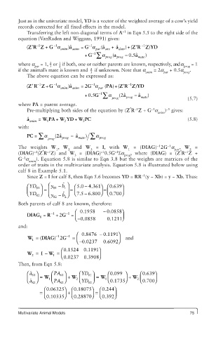
Just as in the univariate model, YD is a vector of the weighted average of a cow’s yield
records corrected for all fixed effects in the model.
−1
Transferring the left non-diagonal terms of A in Eqn 5.5 to the right side of the
equation (VanRaden and Wiggans, 1991) gives:
−
−
1
1
( ′ − 1 + G a anim )a ˆ anim = G a par (a ˆ sire + a ˆ dam )+( ′ − 1 )
ZR Z YD
ZR Z
+ + G − 1 ∑ a prog a ( prog − 0.5a ˆ mate )
2 1
3
par 2 prog
where a = 1, or if both, one or neither parents are known, respectively, and a = 1
2 .
3 anim par prog
if the animal’s mate is known and if unknown. Note that a = 2a + 0.5a
The above equation can be expressed as:
−
−
1
( ′ − 1 + G a anim )a ˆ anim = 2G a par (PA )+(Z R Z′ − 1 )YD
1
ZR Z
− 1
+0.5G ∑ a prrog (2ˆ a prog − ˆ a mate ) (5.7)
where PA = parent average.
−1
−1 −1 ) gives:
Pre-multiplying both sides of the equation by (Z ′ R Z + G a anim
+
+
ˆ a = W PA W YD W PC (5.8)
anim 1 2 3
with:
PC = ∑ a prog ( 2a ˆ prog − a ˆ mate ) ∑ a prog
−1 −1 , W =
1
3
1
2
The weights W , W and W = I, with W = (DIAG) 2G a par 2
−1
−1 −1 −1 −1 , where (DIAG) = (Z ′ R Z +
3
(DIAG) (Z ′ R Z) and W = (DIAG) 0.5G Sa prog
−1 ). Equation 5.8 is similar to Eqn 3.8 but the weights are matrices of the
G a anim
order of traits in the multivariate analysis. Equation 5.8 is illustrated below using
calf 8 in Example 5.1.
−1
Since Z = I for calf 8, then Eqn 5.6 becomes YD = RR (y − Xb) = y − Xb. Thus:
⎛ YD ⎞ ⎛ y 81 − b ˆ 1 ⎞ ⎛ . − . . ⎞
50 4361⎞ ⎛0 639
=
81
⎜ ⎝ YD ⎠ ⎟ = ⎜ ⎜ ⎝ y 82 − b ⎠ ⎟ = ⎜ ⎜ ⎝ . − . ⎟ ⎜ ⎟ ⎠
⎟
ˆ
75 6800⎠ ⎝0 700.
82
2
Both parents of calf 8 are known, therefore:
⎛ 0.1958 − 0.0858⎞
DIAG = R − 1 + 2 G − 1 = ⎜ ⎝ − 0.0858 0.1211⎠ ⎟
8
and:
0 1191⎞
⎛ 0 8476 − .
.
W = ( DIAG) − 1 2 G − 1 = ⎜ ⎟ and
1 ⎝ − 0 0237 0 6092⎠
.
.
⎛0 1524. 0 1191 ⎞
.
=
W = I − W =
2 1 ⎜ ⎝0 0237. 0 3908 ⎟ ⎠
.
Then, from Eqn 5.8:
⎛ ˆ a ⎞ ⎛ PA ⎞ ⎛ YD ⎞ ⎛ . 0 099 ⎞ ⎛ .
0 639⎞
81
81
81
⎜ ⎝ ˆ a ⎠ ⎟ = W 1 ⎜ ⎝ PA ⎠ ⎟ + W 2 ⎜ ⎝Y D ⎠ ⎟ = W 1 ⎜ ⎝ . 0 11735⎠ ⎟ + W 2 ⎜ ⎝ . ⎟
0 700⎠
82
82
82
0 06325⎞
⎛ . ⎛ 0 180755⎞ ⎛ 0 244⎞
.
.
= ⎜ ⎝ . ⎟ + ⎜ ⎝ 0 28870⎠ ⎟ = ⎜ ⎝ 0 392⎠ ⎟
0 10335⎠
.
.
Multivariate Animal Models 75