Page 94 - Linear Models for the Prediction of Animal Breeding Values 3rd Edition

−1
Thus for computational ease, pre-multiply W with G , and the equation for
2prog
DYD becomes:
∑ − 1 YD u ˆ − 1
−
DYD = G W 2 prog a prog (2 mate ) G W 2 prog a prog
−1
The product of G W is symmetric and only upper or lower triangular elements
2prog
need to be stored. The computation of DYD is illustrated in Section 5.4.2, using the
example dairy data.

5.3 Equal Design Matrices with Missing Records

When all traits in a multivariate analysis are not observed in all animals, the same
methodology described in Section 5.2 can also be employed to evaluate animals,
except that different residual covariance matrices have to be set up corresponding to
a different combination of traits present. If the loss of traits is sequential, that is, the
presence of the ith record implies the presence of 1 to (i − 1) records, then the number
of residual covariance matrices is equal to the number of traits. In general, if there are
n
n traits, there are (2 − 1) possible combinations of observed traits and therefore
residual covariance matrices (Quaas, 1984).

5.3.1 An illustration

Example 5.2
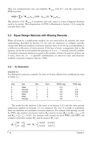
For illustrative purposes, consider the data set below, obtained by modifying the data
in Table 5.1.

Calf Sex Sire Dam WWG (kg) PWG (kg)
4 Male 1 – 4.5 –
5 Female 3 2 2.9 5.0
6 Female 1 2 3.9 6.8
7 Male 4 5 3.5 6.0
8 Male 3 6 5.0 7.5
9 Female 7 – 4.0 –

The model for the analysis is the same as in Section 5.2.1 and the same genetic
parameters applied in Example 5.1 are assumed. The loss of records is sequential;
there are therefore two residual covariance matrices. For animals with missing records
−1
for PWG, the residual covariance matrix (R ) and its inverse (R ) are R = r m11 = 40
m
m
m
1
11
−1
and R = r = = 0.025. For animals with records for both WWG and PWG, the
m m 40
−1
residual covariance matrix (R ) and its inverse (R ) are:
o o
⎡ 40 11⎤ ⎡ 0.028 − 0.010⎤ ⎤
o =
R o = ⎢ ⎥ and R −1 ⎢ ⎥
⎣ 11 30 ⎦ ⎣ − 0.010 0.037 ⎦
78 Chapter 5