Page 97 - Linear Models for the Prediction of Animal Breeding Values 3rd Edition

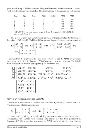
yield in each parity as different traits and fitting a different HYS effect for each trait. The data
with each lactational yield treated as different traits and HYS recoded for each trait is:

Cow Sire Dam HYS1 HYS2 FAT1 FAT2
4 1 2 1 1 201 280
5 3 2 1 2 150 200
6 1 5 2 1 160 190
7 3 4 1 1 180 250
8 1 7 2 2 285 300

HYS1, HYS2, herd–year–season for parity 1 and 2, respectively; FAT1, FAT2, fat
yield in parity 1 and 2.
The aim is to carry out a multivariate estimate of breeding values for fat yield in
lactation 1 (FAT1) and 2 (FAT2) as different traits. Assume the genetic parameters are:
⎡ 65 27⎤ ⎡ 35 28⎤ − 1 ⎡ 0.018 − 0.0007⎤
R = ⎢ ⎥ and G = ⎢ ⎥ with R = ⎢ ⎥ and
⎣ 27 70 ⎦ ⎣ 28 30 ⎦ ⎣ − 0.007 0.017 ⎦
⎡ 0.113 − 0.105⎤
G −1 = ⎢ ⎥
⎣ − 0.105 0.132 ⎦

The model for the analysis is the same as in Section 5.2 but the MME are different
from those in Section 5.2 because HYS effects are peculiar to each trait. The MME
with the equations written out separately for each trait are:

′
12
11
ˆ ⎡ 1 b ⎤ ⎡ X RX 1 X′ 1 R X 2 X′ 1 R Z 1 X′ 1 RRZ 2 ⎤ − 1
11
12
1
⎢ ⎥ ⎢ ′ 21 ′ 22 ′ 21 ′ 22 ⎥
⎢ ˆ 2 b ⎥ = ⎢ XR X 1 X R X 2 X R Z 1 X R Z 2 ⎥
2
2
2
2
−
′
′
−
′
⎢ 1 ˆ a ⎥ ⎢ ZR X 1 Z R X 2 ZR Z 1 1 A g Z′ 1 R Z 2 A g 12 ⎥
11
1
1 11
12
12
11
+
+
1
1
⎢ ⎥ ⎢ 1 ⎥
2 ˆ a ⎣ ⎦ ⎢ ⎣ Z′ 2 RX 1 Z ′ 2 R X 2 Z′ 2 R Z 1 A g Z′′ 2 RZ 2 A g ⎦ ⎥
−
22
21
21
−1
22
1 21
22
+
+
⎡ XR 11 y + XR 12 y ⎤
′
′
⎢ 1 1 1 2 ⎥
′
⎢ XR 21 y+ ′ R 22 2 2 y ⎥
1 X
2
2
⎢ 11 12 ⎥
′
⎢ ZR y+ Z′ 1 R 2 y ⎥
1
1
⎢ ′ 21 y+ ′ 22 ⎥
⎣ ZR 1 Z R 2 y ⎦
2
2
SETTING UP THE DESIGN MATRICES AND MME
The matrix X now relates HYS effects to FAT1 while X relates HYS effects to FAT2.
1 2
The transposes of these matrices are:
é 11 0 1 0ù é 10 1 1 0ù
X¢ = ê ú and X¢ = ê ú
1
2
ë 00 1 0 1 û ë 01 0 0 1 û
Matrices Z and Z are equal and they are identity matrices of order 5 by 5
1 2
−1
considering only animals with records. The matrix A has been presented in
Section 4.2.2. The remaining matrices in the MME can be obtained as described in
Multivariate Animal Models 81