Page 88 - Linear Models for the Prediction of Animal Breeding Values 3rd Edition

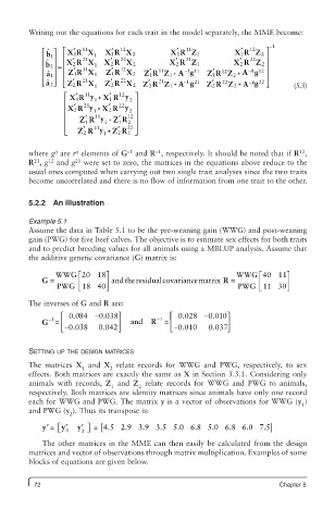
Writing out the equations for each trait in the model separately, the MME become:

′
′
11
ˆ ⎡ 1 b ⎤ ⎡ XR X X ′ 1R X 2 X ′ 1R Z 1 X 1RRZ 2 ⎤ − 1
11
12
12
1
⎢ ˆ ⎥ ⎢ XR X 1 ′ 22 ′ 21 ′ 22 ⎥
′
21
2
⎢ 2 b ⎥ = ⎢ 2 ′ 11 1 X R X 2 X R Z 1 X R Z 2 ⎥
2
2
′
′
−
12
−
1
11
12
1
⎢ 1 ˆ a ⎥ ⎢ ZR X 1 Z R X 2 ZR Z 1 1 A g 11 Z ′ 1R Z 2 + A g ⎥
12
+
1
1
1
⎢ 2 ˆ a ⎣ ⎥ ⎢ ZR X 1 Z ′ 2R X 2 ZR Z 1 A g 21 Z ′′ 2 RZ 2 A g 22 ⎥ ⎦ (5.3)
′
′
21
22
−
21
−
1
⎦ ⎣
1
22
+
+
2
2
′
′
⎡ XR y + XR y ⎤
12
11
1
1
⎢ ′ 21 1 ′ 22 2 ⎥
⎢ XR y 1 + XR y 2 2 ⎥
2
2
′
′
⎢ ZR y + Z R ⎥
12
11
⎢ 1 21 1 1 2 22 ⎥
′
⎣ ZR y 1 + Z ′ 2 R ⎦
2
2
−1
12
−1
ij
ij
where g are r elements of G and R , respectively. It should be noted that if R ,
12
R , g and g were set to zero, the matrices in the equations above reduce to the
21
21
usual ones computed when carrying out two single trait analyses since the two traits
become uncorrelated and there is no flow of information from one trait to the other.
5.2.2 An illustration
Example 5.1
Assume the data in Table 5.1 to be the pre-weaning gain (WWG) and post-weaning
gain (PWG) for five beef calves. The objective is to estimate sex effects for both traits
and to predict breeding values for all animals using a MBLUP analysis. Assume that
the additive genetic covariance (G) matrix is:
é
WWG é20 18 ù WWG 40 11ù
G = ê ú andtheresidualcovariancematrix R = ê ú
PWG 18 40 û P PWG 11 30 û
ë
ë
The inverses of G and R are:
⎡ 0.0 84 −0.038 ⎤ ⎡ 0.028 −0.01 0⎤
−1
−1
G = ⎢ ⎥ and R = ⎢ ⎥
⎣ −0.038 0.042 ⎦ ⎣ −0.0110 0.037 ⎦
SETTING UP THE DESIGN MATRICES
The matrices X and X relate records for WWG and PWG, respectively, to sex
1 2
effects. Both matrices are exactly the same as X in Section 3.3.1. Considering only
animals with records, Z and Z relate records for WWG and PWG to animals,
1 2
respectively. Both matrices are identity matrices since animals have only one record
each for WWG and PWG. The matrix y is a vector of observations for WWG (y )
1
and PWG (y ). Thus its transpose is:
2
′ y = ⎡y ′ y ′ ⎤ [4.5 2.9 3.9 3.5 5.0 6.8 5.0 6.8 6.0 7.5 ]
=
⎦
⎣ 1 2
The other matrices in the MME can then easily be calculated from the design
matrices and vector of observations through matrix multiplication. Examples of some
blocks of equations are given below.
72 Chapter 5