Page 78 - Linear Models for the Prediction of Animal Breeding Values 3rd Edition

2
2
2
between records of an individual is referred to as repeatability and is (s + s )/s .
g pe y
Genetic evaluation under this model is concerned not only with predicting breeding
values but also permanent environmental effects.
4.2.1 Defining the model

The repeatability model is usually of the form:
y = Xb + Za + Wpe + e (4.1)
where y = vector of observations, b = vector of fixed effects, a = vector of random
animal effects, pe = vector of random permanent environmental effects and non-
additive genetic effects, and e = vector of random residual effect. X, Z and W are
incidence matrices relating records to fixed animal and permanent environmental
effects, respectively.
Note that the vector a only includes additive random animal effects; conse-
quently, non-additive genetic effects are included in the pe term. It is assumed that the
permanent environmental effects and residual effects are independently distributed
with means of zero and variance s and s , respectively. Therefore:
2
2
pe e
2
pe
var(pe) = Is
2
var(e) = Is = R
e
2
var(a) = As a
and:
var(y) = ZAZ′s + WIs W′ + R
2
2
a pe
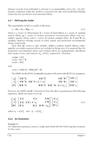
The MME for the BLUE of estimable functions of b and for the BLUP of a and pe are:
–1
¢
¢
¢
–1
¢
–1
é b ˆ ù é XR X X R Z XR W ù é XR yù
–1
–1
ú ê
ú
ê ˆ a = ê ê ¢ –1 ¢ –1 + –1 2 ¢ Z ZR Wú ê ZR ¢ –1 1 yú ú
–1
ê ú ZR X Z R Z A 1/ s a
–1 ú
ê ë ˆ peú û ê ë ê WR X W R Z WR W + I(1 / s 2 ú ê ë WR y û ú
¢
¢
¢
¢
–1
–1
–1
û ú ê
)
pe
−1
However, the MME with R factored out from the above equations give the following
equations, which are easier to set up:
′
′
′ ⎤
ˆ ⎤
⎡ b ⎡ XX XZ ′ XW⎤ –1 ⎡ Xy
⎢ ˆ a = ⎢ −1 ′ ⎥ ⎢ ′ ⎥
⎥
′
⎢ ⎥ ⎢ ⎢ ZX ZZ ′ + A a 1 ZW ⎥ ⎢ Zy ⎥ (4.2)
⎢ ⎣ ˆ pe⎥ ⎦ ⎢ ⎣ WX WZ WW + a 2⎦ ⎥ ⎣ ⎢Wy ⎦
′ ⎥
′
′
′
I
2 2 2 2
1 e a 2 e pe
where a = s /s and a = s /s
4.2.2 An illustration
Example 4.1
For illustrative purposes, assume a single dairy herd with the following data structure
for five cows:
62 Chapter 4