Page 62 - Libro vascular I

Chap-05.qxd 29~8~04 13:25 Page 53
BLOOD FLOW AND ITS APPEARANCE ON COLOR FLOW IMAGING
53
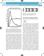
Decrease in cross-sectional area (%) 96 84 64 36
Blood flow
Velocity
600
500
400
300
200
100
0
to quantify the degree of narrowing. Eventually, there comes a point at which the resistance to flow produced by the narrowing is so great that the flow drops to such an extent that the velocity begins to decrease, as shown on the left side of the graph. This is seen as ‘trickle flow’ within the vessel. It is espe- cially important to be able to identify trickle flow within a stenosis as the peak velocities seen may be similar to those seen in healthy vessels, but the color image and waveform shapes will not appear normal.
As blood flow is pulsatile and arteries are non- rigid vessels, it is difficult to predict theoretically the velocity increase that would be seen for a particular diameter reduction. Instead, velocity criteria used to quantify the degree of narrowing are produced by comparing Doppler velocity measurements with arteriogram results, as arteriography is considered to be the ‘gold standard’ for the diagnosis of arterial disease.
Figure 5.5 The change in velocity profile with distance along a vessel from a blunt to a parabolic. (After Caro et al 1978, with permission.)
FLOW PROFILES IN NORMAL ARTERIES
There are three types of flow observed in arteries:
● laminar
● disturbed ● turbulent.
The term laminar flow refers to the fact that the blood cells move in layers, one layer sliding over another, with the different layers being able to move at different velocities. In laminar flow, the blood cells remain in their layers. Turbulent flow occurs when laminar flow breaks down, which is unusual in normal healthy arteries but can be seen in the presence of high-velocity flow caused by stenoses, as discussed later in this chapter.
Figure 5.5 is a schematic diagram showing how the flow profile is expected to change as fluid enters a vessel. When flow enters a vessel from a reservoir (in the case of blood flow, this is the heart), all the fluid is moving at the same velocity, producing a flat velocity profile. This means that the velocity of the fluid close to the vessel wall is similar to that at the center of the vessel. As the fluid flows along the vessel, viscous drag exerted by the walls causes the fluid at the vessel wall to remain motionless, producing a gradient between the velocity in the center of the vessel and that at the walls. As the total flow has to remain constant (as there are no branches in our imaginary tube), the velocity at the center of the vessel will increase to compensate for the low velocity at the vessel wall. This leads to a change in the velocity profile from the initial blunt flow profile to a parabolic flow profile. This is often known as an entrance effect. The distance required for the flow profile to develop from the blunt to the parabolic profile depends on vessel diameter and velocity, but it is
80 60
Decrease in diameter (%)
Changes in flow and velocity as the degree of stenosis alters, predicted by a simple theoretical model of a smooth, symmetrical stenosis. (After Spencer & Reid 1979 Quantitation of carotid stenosis with continuous-wave (C-W) Doppler ultrasound. Stroke 10(3):326–330, with permission.)
40 30 20
Figure 5.4
Velocity (cm/s) or flow (ml/min)