Page 107 - Microeconomics, Fourth Edition

c03consumerpreferencesandtheconceptofutility.qxd 6/14/10 2:54 PM Page 81

3.2 UTILITY FUNCTIONS 81
would decline (e.g., the slope of the total utility curve at point C is negative, and thus
the marginal utility is negative, as indicated at point C ).
Although more may not always be better, it is nevertheless reasonable to assume
that more is better for amounts of a good that a consumer might actually purchase.
For example, in Figure 3.3 we would normally only need to draw the utility function
for the first seven hamburgers. The consumer would never consider buying more than
seven hamburgers because it would make no sense for her to spend money on ham-
burgers that reduce her satisfaction.

PREFERENCES WITH MULTIPLE GOODS:
MARGINAL UTILITY, INDIFFERENCE CURVES,
AND THE MARGINAL RATE OF SUBSTITUTION
Let’s look at how the concepts of total utility and marginal utility might apply to a
more realistic scenario. In real life, consumers can choose among myriad goods and
services. To study the trade-offs a consumer must make in choosing his optimal bas-
ket, we must examine the nature of consumer utility with multiple products.
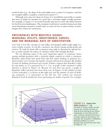
We can illustrate many of the most important aspects of consumer choice
among multiple products with a relatively simple scenario in which a consumer,
Brandon, must decide how much food and how much clothing to purchase in a
given month. Let x measure the number of units of food and y measure the number
of units of clothing purchased each month. Further, suppose that Brandon’s utility
for any basket (x, y) is measured by U 1xy. A graph of this consumer’s utility
function is shown in Figure 3.4. Because we now have two goods, a graph of
Brandon’s utility function must have three axes. In Figure 3.4 the number of units
of food consumed, x, is shown on the right axis, and the number of units of cloth-
ing consumed, y, is represented on the left axis. The vertical axis measures
Brandon’s level of satisfaction from purchasing any basket of goods. For example,

U = 10
12
10 U = 8
U, level of utility 8 U = 4 U = 6 FIGURE 3.4 Graph of the

6

4
The level of utility is shown on the
2 A B C Utility Function U 1xy
vertical axis, and the amounts of
food (x) and clothing (y) are shown,
12
10 respectively, on the right and left
8 U = 2 axes. Contours representing lines of
6 constant utility are also shown. For
4 10 12 example, the consumer is indifferent
2 6 8 between baskets A, B, and C
2 4
y, units of clothing
0 x, units of food because they all yield the same level
of utility (U 4).