Page 50 - Microeconomics, Fourth Edition

c01analyzingeconomicproblems 6/14/10 1:38 PM Page 24

24 CHAPTER 1 ANALYZING ECONOMIC PROBLEMS
9P
s
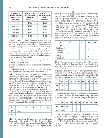
Emissions of Annual Cost Annual Cost given by Q 2 , where T is the average
CO 2 by a Plant of Operating of Operating 1 .05(T 70)
(metric tons Plant 1 Plant 2 temperature (measured in degrees Fahrenheit) in
per year) (millions) (millions) pistachio-growing regions such as Iran. The supply
curve implies that as the temperature deviates from
o
0 $490 $250 the ideal growing temperature of 70 , the quantity of
pistachios supplied goes down. Let P* denote the
250,000 $360 $160
equilibrium price and Q* denote the equilibrium
500,000 $250 $ 90 quantity. Complete the following table showing how
the equilibrium quantity and price vary with the aver-
750,000 $160 $ 40
age temperature. Verify that when T 70, the equilib-
1,000,000 $ 90 $ 10 rium price is $1 per kilogram and the equilibrium
quantity is 9 million kilograms per year.
The firm’s goal is to choose emissions levels at each plant
that minimize its total cost of operating its plants, sub- T 30 50 65 70 80
ject to meeting its emissions target of 1 million metric
tons of CO 2 per year from both plants combined. Let X Q*
denote the quantity of emissions from plant 1 and Y de- (millions of 9
note the quantity of emissions from plant 2. Let TC(X, Y ) kilograms
denote the total operating cost of the firm when the per year)
quantity of emissions from plant 1 is X and the quantity P* ($ per
of emissions from plant 2 is Y. 1
kilogram)
a) What is the objective function for this problem?
b) What is the constraint? 1.20. Consider the comparative statics of the farmer’s
c) Write a statement of the constrained optimization fencing problem in Learning-By-Doing Exercise 1.4,
problem. where L is the length of the pen, W is the width, and
A LW is the area.
d) In light of the information in the table, what emis-
sions levels from each plant should the firm choose? a) Suppose the number of feet of fence given to the farmer
was initially F 1 200. Complete the following table. Verify
1.18. The demand curve for peaches is given by the that the optimal design of the fence (the one yielding the
d
equation Q 100 4P, where P is the price of peaches largest area with a perimeter of 200 feet) would be a square.
d
expressed in cents per pound and Q is the quantity of
peaches demanded (expressed in thousands of bushels per L 10 20 30 40 50 60 70 80 90
s
year). The supply curve for peaches is given by Q RP,
where R is the amount of rainfall (inches per month dur- W 90 80
s
ing the growing season) and Q is the quantity of peaches
supplied (expressed in thousands of bushels per year). Let A 900
P* denote the market equilibrium price and Q* denote
the market equilibrium quantity. Complete the following b) Now suppose the farmer is instead given 240 feet of fence
table showing how the equilibrium quantity and price (F 240). Complete the following table. By how much
vary with the amount of rainfall. Verify that when R 1, would the length L of the optimally designed pen increase?
the equilibrium price is 20 cents per pound and the equi-
librium quantity is 20,000 bushels per year. L 20 30 40 50 60 70 80 90 100

W 100 90
R 1 2 4 8 16
Q* 20 A 2000
P* 20 16.67 c) When the amount of fence is increased from 200 to 240
( F 40), what is the change in the optimal length ( L)?
1.19. The worldwide demand curve for pistachios is d) When the amount of fence is increased from 200 to 240
d
given by Q 10 P, where P is the price of pistachios ( F 40), what is the change in the optimal area ( A)? Is
d
in U.S. dollars and Q is the quantity in millions of kilo- the area A endogenous or exogenous in this example?
grams per year. The world supply curve for pistachios is Explain.