Page 704 - Microeconomics, Fourth Edition

c16GeneralEquilibriumTheory.qxd 8/16/10 9:14 PM Page 678

678 CHAPTER 16 GENERAL EQUILIBRIUM THEORY

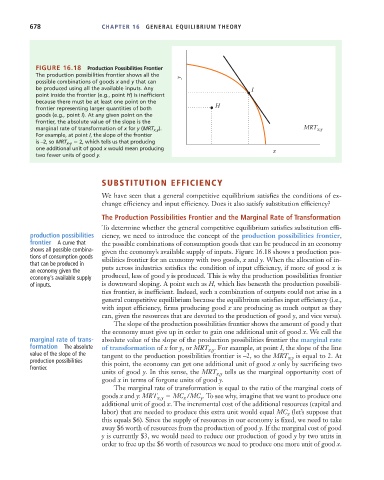
FIGURE 16.18 Production Possibilities Frontier
The production possibilities frontier shows all the
possible combinations of goods x and y that can
be produced using all the available inputs. Any I
point inside the frontier (e.g., point H) is inefficient Quantity of good y
because there must be at least one point on the H
frontier representing larger quantities of both
goods (e.g., point I). At any given point on the
frontier, the absolute value of the slope is the
x,y
marginal rate of transformation of x for y (MRT x,y ). slope = –2, so MRT = 2
For example, at point I, the slope of the frontier
is –2, so MRT x , y 2, which tells us that producing
one additional unit of good x would mean producing 0 Quantity of good x
two fewer units of good y.

SUBSTITUTION EFFICIENCY
We have seen that a general competitive equilibrium satisfies the conditions of ex-
change efficiency and input efficiency. Does it also satisfy substitution efficiency?
The Production Possibilities Frontier and the Marginal Rate of Transformation
To determine whether the general competitive equilibrium satisfies substitution effi-
production possibilities ciency, we need to introduce the concept of the production possibilities frontier,
frontier A curve that the possible combinations of consumption goods that can be produced in an economy
shows all possible combina- given the economy’s available supply of inputs. Figure 16.18 shows a production pos-
tions of consumption goods sibilities frontier for an economy with two goods, x and y. When the allocation of in-
that can be produced in puts across industries satisfies the condition of input efficiency, if more of good x is
an economy given the
economy’s available supply produced, less of good y is produced. This is why the production possibilities frontier
of inputs. is downward sloping. A point such as H, which lies beneath the production possibili-
ties frontier, is inefficient. Indeed, such a combination of outputs could not arise in a
general competitive equilibrium because the equilibrium satisfies input efficiency (i.e.,
with input efficiency, firms producing good x are producing as much output as they
can, given the resources that are devoted to the production of good y, and vice versa).
The slope of the production possibilities frontier shows the amount of good y that
the economy must give up in order to gain one additional unit of good x. We call the
marginal rate of trans- absolute value of the slope of the production possibilities frontier the marginal rate
formation The absolute of transformation of x for y, or MRT . For example, at point I, the slope of the line
x,y
value of the slope of the tangent to the production possibilities frontier is –2, so the MRT x,y is equal to 2. At
production possibilities this point, the economy can get one additional unit of good x only by sacrificing two
frontier.
units of good y. In this sense, the MRT x,y tells us the marginal opportunity cost of
good x in terms of forgone units of good y.
The marginal rate of transformation is equal to the ratio of the marginal costs of
goods x and y: MRT x, y MC /MC . To see why, imagine that we want to produce one
y
x
additional unit of good x. The incremental cost of the additional resources (capital and
labor) that are needed to produce this extra unit would equal MC (let’s suppose that
x
this equals $6). Since the supply of resources in our economy is fixed, we need to take
away $6 worth of resources from the production of good y. If the marginal cost of good
y is currently $3, we would need to reduce our production of good y by two units in
order to free up the $6 worth of resources we need to produce one more unit of good x.