Page 709 - Microeconomics, Fourth Edition

c16GeneralEquilibriumTheory.qxd 8/16/10 9:14 PM Page 683

16.5 GAINS FROM FREE TRADE 683

TABLE 16.1 Labor Requirements in the United States and Mexico
Computers (labor-hours per unit) Clothing (labor-hours per unit)
United States 10 5
Mexico 60 10

For example, Table 16.1 says that in the United States it takes 10 labor-hours to
produce 1 computer, while in Mexico it takes 60 labor hours to produce that com-
puter. Similarly, in the United States it takes 5 labor-hours to produce 1 unit of cloth-
ing, while in Mexico it takes 10 labor-hours to do so. Notice that Table 16.1 implies
that U.S. workers are more productive in both computer and clothing production
than their Mexican counterparts since it takes fewer U.S. labor-hours to make a unit
of either product.
Let’s assume that, in each country, there are 100 available labor-hours each week.
With the numbers in Table 16.1, we can draw the production possibilities frontiers for
the United States and Mexico. These are shown in Figure 16.21. For the United
States, the marginal rate of transformation of computers for clothing is 10/5, or 2.
This is because for every additional computer that is produced, 10 additional labor-
hours are required. With the supply of labor fixed, these 10 labor-hours would have
to be diverted from clothing production, which then means that 2 fewer units of
clothing can be produced. Put another way, in the United States, the opportunity cost

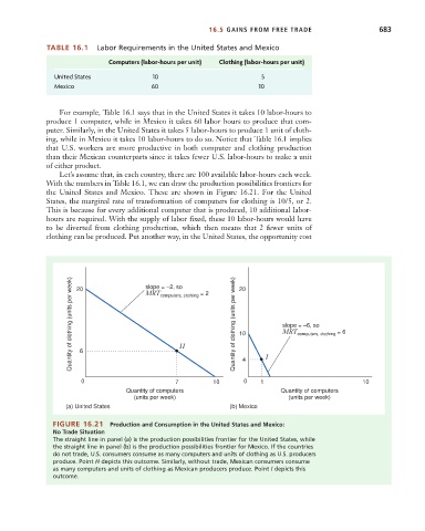
Quantity of clothing (units per week) 20 6 slope = –2, so = 2 Quantity of clothing (units per week) 20 slope = –6, so = 6
MRT
computers, clothing

MRT
10
computers, clothing
H

0 7 10 4 0 1 I 10
Quantity of computers Quantity of computers
(units per week) (units per week)
(a) United States (b) Mexico
FIGURE 16.21 Production and Consumption in the United States and Mexico:
No Trade Situation
The straight line in panel (a) is the production possibilities frontier for the United States, while
the straight line in panel (b) is the production possibilities frontier for Mexico. If the countries
do not trade, U.S. consumers consume as many computers and units of clothing as U.S. producers
produce. Point H depicts this outcome. Similarly, without trade, Mexican consumers consume
as many computers and units of clothing as Mexican producers produce. Point I depicts this
outcome.