Page 360 - Fiber Optic Communications Fund

Performance Analysis 341

x 1 (T b * t) If r(T b ) > r T
+ select x 1 (t)
y(t) t = T b Threshold
∑
r(t) r(T b ) device
* If r`(T b ) < r T
x 0 (T b * t) select x 0 (t)
h(t)

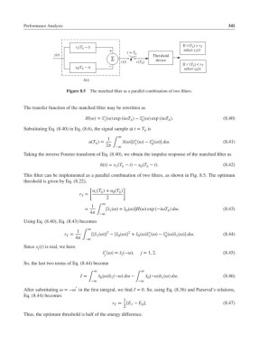
Figure 8.5 The matched filter as a parallel combination of two filters.

The transfer function of the matched filter may be rewritten as
∗ ∗
H()= ̃x () exp (iT )− ̃x () exp (iT ). (8.40)
1 b 0 b
Substituting Eq. (8.40) in Eq. (8.6), the signal sample at t = T is
b
∞
1 ∗ ∗
u(T )= 2 ∫ −∞ ̃ x()[̃x ()− ̃x ()] d. (8.41)
b
0
1
Taking the inverse Fourier transform of Eq. (8.40), we obtain the impulse response of the matched filter as
h(t)= x (T − t)− x (T − t). (8.42)
b
b
0
1
This filter can be implemented as a parallel combination of two filters, as shown in Fig. 8.5. The optimum
threshold is given by Eq. (8.22),
[ ]
u (T )+ u (T )
1
b
0
b
r =
T
2
∞
1
= [̃x ()+ ̃x ()]H() exp (−iT ) d. (8.43)
4 ∫ 1 0 b
−∞
Using Eq. (8.40), Eq. (8.43) becomes
∞
1 2 2 ∗ ∗
r = 4 ∫ −∞ [|̃x ()| − |̃x ()| + ̃x ()̃x ()− ̃x ()̃x ()] d. (8.44)
0
1
0
T
1
1
0
Since x (t) is real, we have
j
∗
̃ x ()= ̃x (−), j = 1, 2. (8.45)
j j
So, the last two terms of Eq. (8.44) become
∞ ∞
I = ̃ x ()̃x (−) d − ̃ x (−)̃x () d. (8.46)
0
∫ ∫
1
0
1
−∞ −∞
′
After substituting =− in the first integral, we find I = 0. So, using Eq. (8.36) and Parseval’s relations,
Eq. (8.44) becomes
1
r = [E − E ]. (8.47)
T
1
0
2
Thus, the optimum threshold is half of the energy difference.