Page 504 - Fiber Optic Communications Fund

Nonlinear Effects in Fibers 485

Δ −2,1,−1 = 0.5 + 0.8 −(−0.7) rad
= 2 rad, (10.454)

P(dBm)= 3 dBm, (10.455)

P(mW)= 10 P(dBm)∕10 mW
= 2 mW. (10.456)

Substituting Eqs. (10.453), (10.454), and (10.456) in Eq. (10.452), we find
√
(−2,1,−1,0) −4
(L)=(−0.8 + 1.6i)× 10 W. (10.457)
0
Similarly, the FWM fields due to other triplets are
√
(−2,2,0,0) −7 −5
(L)=(3.33 × 10 − 3.92 × 10 i) W, (10.458)
0
√
(−1,−1,−2,0) −4
(L)=(2.03 + 1.9i)× 10 W, (10.459)
0
√
(−1,1,0,0) −4
(L)=(2.28 − 1.6i)× 10 W, (10.460)
0
√
(−1,2,1,0) −4
(L)=(−1.4 − 1.12 i)× 10 W, (10.461)
0
√
(1,1,2,0) −4
(L)=(1.435 − 2.394 i)× 10 W. (10.462)
0
The total FWM field is
= 2 (−2,1,−1,0) + 2 (−2,2,0,0) + 2 (−1,1,0,0) + 2 (−1,2,1,0) + (1,1,2,0) + (−1,−1,−2)
0
√
=(3.64 − 3.509 i)× 10 −4 W. (10.463)
The FWM power at the fiber output is
2
P = | | = 2.56 × 10 −4 mW. (10.464)
FWM 0
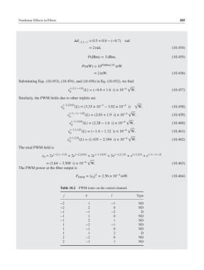
Table 10.2 FWM tones on the central channel.
j k l Type
−2 1 −1 ND
−2 2 0 ND
−1 −1 −2 D
−1 1 0 ND
−1 2 1 ND
1 −2 −1 ND
1 −1 0 ND
1 1 2 D
2 −2 0 ND
2 −1 1 ND