Page 507 - Fiber Optic Communications Fund

488 Fiber Optic Communications

where G = exp ( L ) is the power gain of the amplifier. Comparing Eqs. (10.480) and (10.481), we find
0 a
√
A = G − 1. (10.482)
Substituting Eq. (10.475) in Eq. (10.471), we find

2
da u (Z) u 2 2 (Z)
2
iu + ia − a + a |q| q =−i au
dZ Z 2 T 2 2
N
√ ∑
+i( G − 1) (Z − nL )a(nL )u(T, nL ). (10.483)
a−
a−
a
n=1
Let
N
da −au √ ∑
u = +( G − 1) (Z − nL )a(nL )u(T, nL ), (10.484)
a
a−
a−
dZ 2
n=1
so that Eq. (10.483) becomes
2
u u 2 2
2
i − + a (Z)|u| u = 0. (10.485)
Z 2 T 2
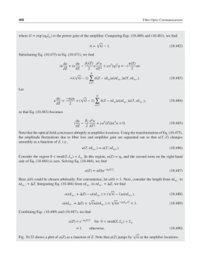
Note that the optical field q increases abruptly at amplifier locations. Using the transformation of Eq. (10.475),
the amplitude fluctuations due to fiber loss and amplifier gain are separated out so that u(T, Z) changes
smoothly as a function of Z, i.e.,
u(T, nL )= u(T, nL ). (10.486)
a− a+
Consider the region 0 < mod(Z, L ) < L . In this region, (Z)= and the second term on the right-hand
0
a
a
side of Eq. (10.484) is zero. Solving Eq. (10.484), we find
− 0 Z∕2
a(Z)= a(0)e . (10.487)
Here a(0) could be chosen arbitrarily. For convenience, let a(0)= 1. Next, consider the length from nL a− to
nL a− +ΔZ. Integrating Eq. (10.484) from nL a− to nL a− +ΔZ, we find
√
a(nL a− +ΔZ)− a(nL )=( G − 1)a(nL ), (10.488)
a−
a−
√ √
a(nL a− +ΔZ)= Ga(nL )= Ge − 0 L a ∕2 = 1. (10.489)
a−
Combining Eqs. (10.489) and (10.487), we find

a(Z)= e − 0 Z∕2 for 0 < mod(Z, L ) < L a
a
= 1 otherwise. (10.490)
√
Fig. 10.33 shows a plot of a(Z) as a function of Z. Note that a(Z) jumps by G at the amplifier locations.