Page 534 - Fiber Optic Communications Fund

Digital Signal Processing 515

ˆ
Ψ in [k] Fiber-optic Ψ out [k] Adaptive Ψ in [k]
Channel equalizer
H W

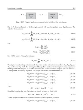
Figure 11.19 Adaptive equalization of the polarization-multiplexed fiber-optic channel.

Fig. 11.19 shows a schematic of the fiber-optic channel with adaptive equalizer in the digital domain. The
output of the equalizer is

K
∑
̂ x,in [n]= F {W [k] x,out [n − k]+ W [k] y,out [n − k]}, (11.96)
xy
xx
k=−K
K
∑
̂ y,in [n]= F {W [k] x,out [n − k]+ W [k] y,out [n − k]}. (11.97)
yx
yy
k=−K
Let
[ ]
̂ x,in [k]
̂
Ψ [k]= , (11.98)
in ̂ y,in [k]
[ ]
W [k] W [k]
xy
xx
W[k]= (11.99)
W [k] W [k].
yy
yx
Eqs. (11.96) and (11.97) may be written as
K
∑
̂
Ψ [n]= W[k]Ψ [x − k]. (11.100)
in
out
k=−K
The adaptive equalizer for polarization mode dispersion consists of four transversal filters, W , W , W , and
xx xy yx
W , as shown in Fig. 11.20. The tap weights of the equalizer can be updated using the training sequence or
yy
blind equalization techniques, as described previously. Let us first consider an adaptive equalizer that uses a
LMS algorithm and training sequences. The weights are updated as (see Example 11.4)
∗
W [k] (n+1) = W [k] (n) + x,out [n − k]e [n]Δ, (11.101)
x
xx
xx
W [k] (n+1) = W [k] (n) + ∗ [n − k]e [n]Δ, (11.102)
xy xy y,out x
∗
W [k] (n+1) = W [k] (n) + y,out [n − k]e [n]Δ, (11.103)
y
yy
yy
∗
W [k] (n+1) = W [k] (n) + x,out [n − k]e [n]Δ, (11.104)
y
yx
yx
where
e [n]= [n]− ̂ [n], r = x, y. (11.105)
r r,in r,in
For a blind equalizer that uses CMA, the error signals are given by Eq. (11.84),
′
2
e [k]= ̂ [k](1 − | ̂ [n]| ), r = x, y. (11.106)
r r,in r,in
The tap weights are adjusted in accordance with the stochastic gradient algorithm,
′
∗
W [k] (n+1) = W [k] (n) + x,out [n − k]e [n]Δ, (11.107)
xx
xx
x