Page 532 - Fiber Optic Communications Fund

Digital Signal Processing 513

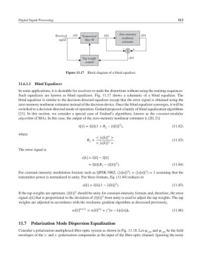
Received y[k] Transversal ˆ x[k] Zero-memory ˜ x[k]
signal filter W nonlinear
estimator
* +

Tap weight e[k]
control

Figure 11.17 Block diagram of a blind equalizer.

11.6.1.1 Blind Equalizers
In some applications, it is desirable for receivers to undo the distortions without using the training sequences.
Such equalizers are known as blind equalizers. Fig. 11.17 shows a schematic of a blind equalizer. The
blind equalizer is similar to the decision-directed equalizer except that the error signal is obtained using the
zero-memory nonlinear estimator instead of the decision device. Once the blind equalizer converges, it will be
switched to a decision-directed mode of operation. Godard proposed a family of blind equalization algorithms
[21]. In this section, we consider a special case of Godard’s algorithms, known as the constant-modulus
algorithm (CMA). In this case, the output of the zero-memory nonlinear estimator is [20, 21]
2
̃ x[k]= ̂x[k](1 + R − |̂x[k]| ), (11.82)
2
where
4
< |x[k]| >
R = . (11.83)
2
2
< |x[k]| >
The error signal is
e[k]= ̃x[k]− ̂x[k]
2
= ̂x[k](R − |̂x[k]| ). (11.84)
2
2
4
For constant-intensity modulation formats such as QPSK-NRZ, ⟨|x[n]| ⟩ = ⟨|x[n]| ⟩ = 1 assuming that the
transmitter power is normalized to unity. For these formats, Eq. (11.84) reduces to
2
e[k]= ̂x[k](1 − |̂x[k]| ). (11.85)
2
If the tap weights are optimum, |̂x[k]| should be unity for constant-intensity formats and, therefore, the error
2
signal e[k] that is proportional to the deviation of |̂x[k]| from unity is used to adjust the tap weights. The tap
weights are adjusted in accordance with the stochastic gradient algorithm as discussed previously,
∗
[k] (n+1) = [k] (n) + y [n − k]e[n]Δ. (11.86)

11.7 Polarization Mode Dispersion Equalization

Consider a polarization-multiplexed fiber-optic system as shown in Fig. 11.18. Let x,in and y,in be the field
envelopes of the x- and y- polarization components at the input of the fiber-optic channel. Ignoring the noise