Page 531 - Fiber Optic Communications Fund

512 Fiber Optic Communications

gradient vector is approximated by the instantaneous value or an estimate of the gradient vector. Ignoring the
expectation operator in Eq. (11.78), the tap weights are altered at the (n + 1)th iteration as [18–20]
∗
W[k] (n+1) = W[k] (n) + y [n − k]e[n]Δ, k =−K, … , 0, … , K (11.79)
e[n]= x[n]− ̂x[n]. (11.80)

Eqs. (11.79) and (11.80) constitute the LMS algorithm for adaptive equalization. After a few iterations,
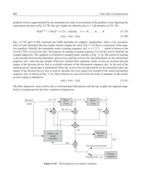
e[n]≅ 0 and, thereafter, the tap weights remain roughly the same. Fig. 11.16 shows a schematic of the adap-
tive equalizer. Initially, the transmitter sends a training sequence x[n], n = 1, 2, 3, … which is known to the
receiver. This is received as y[n]. The purpose of sending a training sequence is to let the receiver find the tap
weights adaptively. The equalizer is switched to training mode, initially in Fig. 11.16. The period of training
is pre-decided between the transmitter and receiver, and the receiver has full information on the information
sequence x[n]. After the tap weights W[k] have reached their optimum values, it may be assumed that the
output of the decision device ̂x[n] is a reliable estimate of the information sequence x[n]. At the end of the
training period, actual data is transmitted. Since the receiver has no information on the transmitted data, the
output of the decision device ̃x[n] is used to calculate the error signal e[n] instead of the actual information
sequence x[n], as shown in Fig. 11.16. This is known as a decision-directed mode of adaption. In this mode,
an error signal is obtained as
e[n]= ̃x[n]− ̂x[n]. (11.81)

The fiber dispersion varies slowly due to environmental fluctuations and the tap weights are adjusted adap-
tively to compensate for the slow variations in dispersion.

Received y[n + K] Delay y[n + K * 1] Delay y[n * K]
T T
signal samp samp
W[* K] W[*K + 1] W[K]
× × ×

ˆ x[n]
Adaptive tap Decision
weight device
controller x[n]
˜
*
e[n]

Decision-directed mode
+
Training
Training mode x []n sequence

Figure 11.16 Block diagram of an adaptive equalizer.